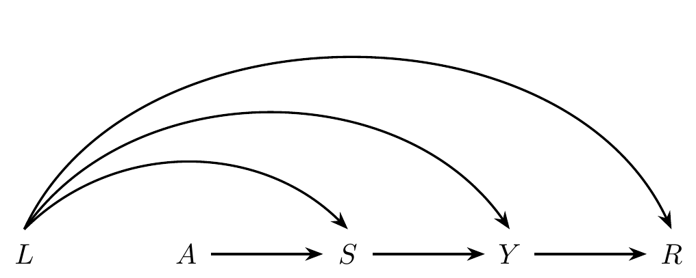
2 Stochastic-interventional vaccine efficacy

In a nutshell

We estimate how vaccine efficacy would change had the vaccine shifted everyone’s antibody titers. In our simulated trial, titers were measured only in a case-cohort sample, so we use lmtp with weights for the sampling design.

Roadmap: (1) the population mean under a modified treatment policy (MTP), the SVE, and its linear-model analogue → (2) one MTP, with misspecified and correct outcome GLMs and Super Learner → (3) the SVE curve → (4) plug-in g-computation, and why it is more fragile → (5) what happens if the sampling design is ignored → (6) positivity.

Notation for this part

Symbol	Meaning
$L$	age, high-risk behaviour, sex
$A$	vaccine (1) or placebo (0), randomized
$Y$	infection by the end of follow-up
$S$	immune marker ($\log_{10}$ antibody titer), a mediator of $A \to Y$
$R$, $g_{0,R}(Y, L)$	phase-two sampling indicator, and its known probability $\P_0(R = 1 \mid Y, L)$
$\overline{Q}_{0,Y}(s, l)$	risk among vaccinees, $\P_0(Y = 1 \mid S = s, A = 1, L = l)$
$g_{0,S}(s \mid l)$	density of $S$ given $A = 1$ and $L = l$ (generalized propensity score)
$d(S, L) = S + \delta$	the modified treatment policy (MTP): an additive shift of $S$
$\psi_{0,\delta}$	population mean under the MTP, $\E_0[Y(d(S, L)) \mid A = 1]$
$\text{SVE}_\delta$	$1 - \psi_{0,\delta} / \P_0(Y = 1 \mid A = 0)$

2.1 The question

In vaccine trials, an immune correlate of protection is a marker of the vaccine-induced immune response $S$ (e.g., neutralizing antibody titer) that tracks protection against the outcome $Y$ (e.g., infection) (Plotkin and Gilbert 2012). Correlates help us understand how a vaccine protects and can serve as surrogate endpoints for future trials (Prentice 1989; Gilbert et al. 2024). The question from the keynote:

Plotkin, Stanley A, and Peter B Gilbert. 2012. “Nomenclature for Immune Correlates of Protection After Vaccination.” Clinical Infectious Diseases 54 (11): 1615–17.

Prentice, Ross L. 1989. “Surrogate Endpoints in Clinical Trials: Definition and Operational Criteria.” Statistics in Medicine 8 (4): 431–40.

Gilbert, Peter B, Youyi Fong, Nima S Hejazi, et al. 2024. “Four Statistical Frameworks for Assessing an Immune Correlate of Protection (Surrogate Endpoint) from a Randomized, Controlled, Vaccine Efficacy Trial.” Vaccine 42 (9): 2181–90. https://doi.org/10.1016/j.vaccine.2024.02.071.

How would the risk of infection have changed had the vaccine induced higher, or lower, antibody titers?

The vaccine $A$ is randomized, but $S$ is not: it is a post-treatment variable on the pathway $A \to S \to Y$, a mediator. Questions about intervening on $S$ are questions about mediation.

2.2 The data: a simulated trial with a case-cohort design

Data from the real trials are not public, so we simulate a trial of 10,000 people. The complete data on one person would be $X = (L, A, S, Y)$:

$L$: age (in years), a high_risk behaviour indicator, sex;
$A$: vaccine (1) or placebo (0), randomized 1:1;
$S$: $\log_{10}$ neutralizing antibody titer ($S = 0$, the assay floor, in the placebo arm);
$Y$: infection by the end of follow-up.

The data are generated (in practical/R/sim_vaccine_trial.R) by the structural equations \[ \begin{aligned} \text{age} &\sim \text{Uniform}\{18, \ldots, 75\}, \quad \mathtt{high\_risk} \sim \text{Bernoulli}(0.35), \quad \text{sex} \sim \text{Bernoulli}(0.5), \\ A &\sim \text{Bernoulli}(0.5), \\ S &= A \cdot \{1.4 - 0.02\,(\text{age} - 45) - 0.2\,\mathtt{high\_risk} + U_S\}, \quad U_S \sim \mathcal{N}(0, 0.5^2), \\ Y &\sim \text{Bernoulli}\big(\operatorname{expit}\{-2.3 + 0.025\, (\text{age} - 45) + 0.9\,\mathtt{high\_risk} - 2.2 \min(S, 1.2)\}\big), \\ R &\sim \text{Bernoulli}\big(g_{0,R}(Y, L)\big), \end{aligned} \] with $g_{0,R}$ given below. The vaccine acts on $Y$ only through $S$; the risk of infection falls with titer up to a $\log_{10}$ titer of 1.2 and is flat above it; sex affects nothing.

Assaying blood samples is expensive, so $S$ is measured only in a phase-two sample, indicated by $R \in \{0, 1\}$: a case-cohort design (Prentice 1986), a special case of two-phase sampling (White 1982; Breslow et al. 2003). The investigators choose who enters phase two, and they choose using only $Y$ and $L$: every infected person (case) is sampled, and non-cases are sampled at random within strata of high_risk. The sampling probabilities are therefore known by design, \[ g_{0,R}(Y, L) = \P_0(R = 1 \mid Y, L) = \begin{cases} 1 & \text{if } Y = 1, \\ 0.25 & \text{if } Y = 0 \text{ and } \mathtt{high\_risk} = 1, \\ 0.15 & \text{if } Y = 0 \text{ and } \mathtt{high\_risk} = 0, \end{cases} \] and recorded as g_R. So the observed data unit is \[ O = (L, A, RS, Y, R) \sim \P_0 \in \mathcal{P}, \] where $RS$ is $S$ when $R = 1$ and missing otherwise.

Prentice, Ross L. 1986. “A Case-Cohort Design for Epidemiologic Cohort Studies and Disease Prevention Trials.” Biometrika 73 (1): 1–11.

White, J Emily. 1982. “A Two Stage Design for the Study of the Relationship Between a Rare Exposure and a Rare Disease.” American Journal of Epidemiology 115 (1): 119–28.

Breslow, Norman, Brad McNeney, and Jon A Wellner. 2003. “Large Sample Theory for Semiparametric Regression Models with Two-Phase, Outcome Dependent Sampling.” The Annals of Statistics 31 (4): 1110–39.

Figure 2.1: DAG for the vaccine trial, in time order. The vaccine $A$ is randomized; covariates $L$ confound the effect of the immune marker $S$ on infection $Y$; inclusion $R$ in the phase-two sample depends, by design, only on $Y$ and $L$. (In our simulation, the vaccine acts on $Y$ only through $S$.)

trial <- sim_vaccine_trial()
head(trial)

  age high_risk sex A        S Y R  g_R
1  56         1   1 1 1.635746 0 1 0.25
2  60         0   0 0       NA 0 0 0.15
3  51         0   1 1       NA 0 0 0.15
4  44         0   0 0       NA 0 0 0.15
5  66         0   0 0       NA 0 0 0.15
6  53         1   0 0 0.000000 0 1 0.25

with(trial, table(vaccine = A, infected = Y))

       infected
vaccine    0    1
      0 4247  672
      1 4921  160

with(trial, table(vaccine = A, phase_two = R))

       phase_two
vaccine    0    1
      0 3463 1456
      1 4069 1012

with(trial, table(phase_two = R, infected = Y)) # every case is sampled

         infected
phase_two    0    1
        0 7532    0
        1 1636  832

We focus on vaccine recipients in the phase-two sample:

vax <- subset(trial, A == 1 & R == 1)
nrow(vax)

[1] 1012

mean(vax$Y) # cases are heavily over-represented!

[1] 0.1581028

2.3 The target parameter

Let $\overline{Q}_{0,Y}(s, l) = \P_0(Y = 1 \mid S = s, A = 1, L = l)$ be the risk of infection among vaccinees, and $g_{0,S}(s \mid l)$ the conditional density of $S$ given $A = 1$ and $L = l$ (the generalized propensity score). A modified treatment policy (MTP) replaces each vaccinee’s natural titer $S$ with a new value $d(S, L)$ that may depend on it (Haneuse and Rotnitzky 2013; Dı́az et al. 2023). Here, the MTP is the additive shift $d(S, L) = S + \delta$ (Dı́az and van der Laan 2012). Our target parameter is the stochastic-interventional vaccine efficacy (Hejazi et al. 2021; Gilbert, Fong, et al. 2021), \[ \text{SVE}_{\delta} = 1 - \frac{\psi_{0,\delta}}{\P_0(Y = 1 \mid A = 0)}. \]

Haneuse, Sebastian, and Andrea Rotnitzky. 2013. “Estimation of the Effect of Interventions That Modify the Received Treatment.” Statistics in Medicine 32 (30): 5260–77.

Dı́az, Iván, and Mark J van der Laan. 2012. “Population Intervention Causal Effects Based on Stochastic Interventions.” Biometrics 68 (2): 541–49.

Gilbert, Peter B, Youyi Fong, David Benkeser, et al. 2021. CoVPN COVID-19 Vaccine Efficacy Trial Immune Correlates Statistical Analysis Plan. https://doi.org/10.6084/m9.figshare.13198595.

The numerator $\psi_{0,\delta} = \E_0[Y(d(S, L)) \mid A = 1]$ is a population mean under the MTP: the risk of infection among vaccinees had each vaccinee’s titer been shifted by $\delta$. Under no unmeasured confounding of $S$ and $Y$ given $L$, and positivity, it is identified by \[ \psi_{0,\delta} = \E_0 \left[ \int \overline{Q}_{0,Y}(d(s, L), L) \, g_{0,S}(s \mid L) \, ds \;\middle|\; A = 1 \right]: \] vaccinees with covariates $L$, shift a given unit’s observed titer value by $\delta$ units, and average the vaccinee risk at the shifted titer $s + \delta$ over $L$.
The denominator is the risk of infection had everyone received placebo, $\P_0(Y(0) = 1)$. Since $A$ is randomized, it is identified most simply by the placebo-arm risk, $\P_0(Y = 1 \mid A = 0)$.¹

¹ Randomization also gives the covariate-adjusted identification $\E_0[\P_0(Y = 1 \mid A = 0, L)]$. Estimating the denominator this way uses the prognostic information in $L$ and can improve efficiency; we use the simpler unadjusted estimate.

Gilbert, Peter B, David C Montefiori, Adrian B McDermott, et al. 2021. “Immune Correlates Analysis of the mRNA-1273 COVID-19 Vaccine Efficacy Clinical Trial.” Science 375 (6576): 43–50. https://doi.org/10.1126/science.abm3425.

Hejazi, Nima S, Xiaoying Shen, Lindsay N Carpp, et al. 2023. “Stochastic Interventional Approach to Assessing Immune Correlates of Protection: Application to the COVE mRNA-1273 Vaccine Trial.” International Journal of Infectious Diseases 137: 28–39. https://doi.org/10.1016/j.ijid.2023.09.012.

Huang, Ying, Nima S Hejazi, Bryan Blette, et al. 2023. “Stochastic Interventional Vaccine Efficacy and Principal Surrogate Analyses of Antibody Markers as Correlates of Protection Against Symptomatic COVID-19 in the COVE mRNA-1273 Trial.” Viruses 15 (10): 2029. https://doi.org/10.3390/v15102029.

Gilbert, Peter B, Youyi Fong, Avi Kenny, and Marco Carone. 2023. “A Controlled Effects Approach to Assessing Immune Correlates of Protection.” Biostatistics 24 (4): 850–65. https://doi.org/10.1093/biostatistics/kxac024.

At $\delta = 0$, this is the usual vaccine efficacy; as $\delta$ varies, it traces out how efficacy would change with the vaccine’s immunogenicity. It was one of the immune correlates analyses of the COVE trial of the Moderna mRNA-1273 COVID-19 vaccine (Gilbert, Montefiori, et al. 2021; Hejazi et al. 2023; Huang et al. 2023). Unlike the controlled vaccine efficacy from the keynote (Gilbert et al. 2023), which sets every vaccinee’s titer to the same value $s$, an MTP moves each person’s titer from where it naturally fell.

2.3.1 Exercise 2.1 ✏️

MTPs, linear models, and sampling

Suppose the outcome model is linear: $\overline{Q}_{0,Y}(s, l) = \beta_0 + \beta_1 s + \gamma^\top l$. Show that $\psi_{0,\delta} - \psi_{0,0} = \beta_1 \delta$. What does $\text{SVE}_\delta$ look like as a function of $\delta$?
What goes wrong with the linear model as $\delta$ grows? (Hint: $\psi_{0,\delta}$ is a probability.)
Among the phase-two vaccinees, what is the share of cases, compared to the full vaccine arm? What would happen if we estimated $\psi_{0,\delta}$ from vax as if it were a random sample of vaccinees? How do the weights $1 / g_{0,R}(Y, L)$ fix this?
Positivity for an MTP requires that, for each $l$, the shifted value $s + \delta$ is a value of $S$ that could occur among people with $L = l$. Why is this harder to satisfy for large $|\delta|$?

Solution

$\psi_{0,\delta} = \E_0[\beta_0 + \beta_1 (S + \delta) + \gamma^\top L \mid A = 1] = \psi_{0,0} + \beta_1 \delta$. So $\text{SVE}_\delta = 1 - (\psi_{0,0} + \beta_1 \delta) / \P_0(Y = 1 \mid A = 0)$ is a straight line in $\delta$ with slope $-\beta_1 / \P_0(Y = 1 \mid A = 0)$: the linear model’s $\beta_1$ is the effect of the MTP with $\delta = 1$, just as $\beta_1$ was the ATE in Part 1.
A straight line eventually leaves $[0, 1]$: for large positive $\delta$ (with $\beta_1 < 0$), the predicted risk becomes negative and the SVE exceeds 100%; the model also forces each additional unit of titer to buy the same reduction in risk, whatever the starting titer.
All cases are sampled but only 15–25% of non-cases, so cases are hugely over-represented (compare mean(vax$Y) with the infection rate in the vaccine arm). Ignoring this would badly overestimate risk. Weighting each phase-two person by $1 / g_{0,R}(Y, L)$ makes them stand in for the $1 / g_{0,R}(Y, L)$ people like them in the full trial (inverse probability weighting), recovering the full-cohort target.
Shifting by $\delta$ asks about titers $s + \delta$; for large $|\delta|$, many shifted titers fall outside the range observed among similar people (e.g., below the assay floor, or far above any observed response), so the data contain no information about risk there and any estimate is an extrapolation.

2.4 Estimation with `lmtp`

The lmtp package (Dı́az et al. 2023) implements estimators of population means under MTPs, including our additive shift. lmtp_tmle() estimates the numerator $\psi_{0,\delta}$ by targeted maximum likelihood. It needs two nuisance estimates: $\overline{Q}_{n,Y}$, and an estimate of the density ratio $g_{0,S}(s - \delta \mid l) / g_{0,S}(s \mid l)$, which lmtp obtains by classifying observed versus shifted titers. Both are fit with SuperLearner libraries (learners_outcome, learners_trt). lmtp_tmle() accepts sampling weights through weights, which gives the inverse-probability-weighted version of the estimator for two-phase designs (Rose and van der Laan 2011).²

Dı́az, Iván, Nicholas Williams, Katherine L Hoffman, and Edward J Schenck. 2023. “Nonparametric Causal Effects Based on Longitudinal Modified Treatment Policies.” Journal of the American Statistical Association 118 (542): 846–57. https://doi.org/10.1080/01621459.2021.1955691.

Rose, Sherri, and Mark J van der Laan. 2011. “A Targeted Maximum Likelihood Estimator for Two-Stage Designs.” The International Journal of Biostatistics 7 (1): 1–21.

² The estimator in the txshift package (Hejazi and Benkeser 2020) also augments the weighted estimator with a model for the sampling mechanism, using information on the whole cohort to gain efficiency (Breslow et al. 2009; Hejazi et al. 2021). The reweighted version is valid here because $g_{0,R}$ is known by design.

Hejazi, Nima S, and David C Benkeser. 2020. “txshift: Efficient Estimation of the Causal Effects of Stochastic Interventions in R.” Journal of Open Source Software 5 (54): 2447. https://doi.org/10.21105/joss.02447.

Breslow, Norman E, Thomas Lumley, Christie M Ballantyne, Lloyd E Chambless, and Michal Kulich. 2009. “Using the Whole Cohort in the Analysis of Case-Cohort Data.” American Journal of Epidemiology 169 (11): 1398–405.

Hejazi, Nima S, Mark J van der Laan, Holly E Janes, Peter B Gilbert, and David C Benkeser. 2021. “Efficient Nonparametric Inference on the Effects of Stochastic Interventions Under Two-Phase Sampling, with Applications to Vaccine Efficacy Trials.” Biometrics 77 (4): 1241–53. https://doi.org/10.1111/biom.13375.

In our simulation, the risk of infection falls with titer only up to a threshold ($\log_{10}$ titer of 1.2) and is flat above it. A main-terms logistic regression ("SL.glm") for $\overline{Q}_{0,Y}$ is therefore misspecified; "SL.glm_threshold" (in practical/R/learners.R), which uses $\min(S, 1.2)$ in place of $S$, is correctly specified. For the density ratio, we use a main-terms logistic regression throughout. It is correctly specified here: $S$ given $A = 1$ and $L$ is normal, with a mean linear in $L$ and constant variance, so the log density ratio is linear in $(s, l)$.

2.4.1 Exercise 2.2 💻

One MTP, three outcome models

Estimate $\psi_{0,0.5}$, the risk among vaccinees had every vaccinee’s titer been $0.5$ $\log_{10}$ units (about 3-fold) higher, using for $\overline{Q}_n$ (i) the misspecified GLM, (ii) the correctly specified GLM, and (iii) a Super Learner whose library includes the correct GLM. Compare to the truth, true_sve(0.5).

shift_by <- function(delta) function(data, trt) ___
fit_shift <- function(delta, q_lib, weights = 1 / vax$g_R) {
  lmtp_tmle(
    data = vax,
    trt = "S",
    outcome = "Y",
    baseline = c("age", "high_risk", "sex"),
    shift = shift_by(delta),
    outcome_type = "binomial",
    learners_outcome = q_lib,
    learners_trt = "SL.glm",
    folds = 5,
    weights = weights
  )
}
sl_lib <- c(
  "SL.mean",
  "SL.glm",
  "SL.glm_threshold",
  "SL.glmnet",
  "SL.earth",
  "SL.gam"
)
fits_05 <- list(
  glm_wrong = fit_shift(0.5, "SL.glm"),
  glm_right = fit_shift(0.5, ___),
  super_learner = fit_shift(0.5, ___)
)
sapply(fits_05, function(fit) {
  c(psi = fit$estimate@x, se = fit$estimate@std_error)
})
true_sve(0.5)

Solution

shift_by <- function(delta) function(data, trt) data[[trt]] + delta
fit_shift <- function(delta, q_lib, weights = 1 / vax$g_R) {
  lmtp_tmle(
    data = vax,
    trt = "S",
    outcome = "Y",
    baseline = c("age", "high_risk", "sex"),
    shift = shift_by(delta),
    outcome_type = "binomial",
    learners_outcome = q_lib,
    learners_trt = "SL.glm",
    folds = 5,
    weights = weights
  )
}
sl_lib <- c(
  "SL.mean",
  "SL.glm",
  "SL.glm_threshold",
  "SL.glmnet",
  "SL.earth",
  "SL.gam"
)
fits_05 <- list(
  glm_wrong = fit_shift(0.5, "SL.glm"),
  glm_right = fit_shift(0.5, "SL.glm_threshold"),
  super_learner = fit_shift(0.5, sl_lib)
)
sapply(fits_05, function(fit) {
  c(psi = fit$estimate@x, se = fit$estimate@std_error)
})

      glm_wrong   glm_right super_learner
psi 0.016524739 0.017072059   0.016768437
se  0.002261512 0.002239203   0.002252903

true_sve(0.5)

  delta        psi       sve
1   0.5 0.01630634 0.8830436

All three are close to the truth, including the misspecified GLM. The TML estimator is doubly robust: it is consistent if either $\overline{Q}_{n,Y}$ or the density ratio is consistent, and here the density ratio model is correctly specified. Exercise 2.4 shows what happens without that protection.

2.4.2 Exercise 2.3 💻

The SVE curve

Estimate $\psi_{0,\delta}$ over a grid of values of $\delta$ with the Super Learner, compute $\text{SVE}_{n,\delta}$ using the placebo-arm risk (estimable from the full trial, since $S$ is not needed), and compare to the truth, which we know because we simulated the data (true_sve()).

deltas <- c(-0.5, -0.25, 0, 0.25, 0.5, 0.75)
risk_placebo <- mean(trial$Y[trial$A == ___])
psi_n <- sapply(deltas, function(delta) fit_shift(___)$estimate@x)
sve <- data.frame(
  delta = deltas,
  lmtp = 1 - psi_n / ___,
  truth = true_sve(deltas)$sve
)
sve

Solution

deltas <- c(-0.5, -0.25, 0, 0.25, 0.5, 0.75)
risk_placebo <- mean(trial$Y[trial$A == 0])
psi_n <- sapply(deltas, function(delta) fit_shift(delta, sl_lib)$estimate@x)
sve <- data.frame(
  delta = deltas,
  lmtp = 1 - psi_n / risk_placebo,
  truth = true_sve(deltas)$sve
)
sve

  delta      lmtp     truth
1 -0.50 0.4726627 0.5110695
2 -0.25 0.6384777 0.6742671
3  0.00 0.7464934 0.7813769
4  0.25 0.8215102 0.8466500
5  0.50 0.8770759 0.8830436
6  0.75 0.9097931 0.9012873

The estimated curve has the shape of the truth but sits a few points below it for most shifts. At $\delta = 0$, the SVE is just the observed vaccine efficacy, which in this sample falls below its true value by chance. For the largest shift, the estimate overtakes the truth: more vaccinees are shifted beyond the titers observed among people like them. This is a first sign of the positivity strain explored in Exercise 2.6a.

2.4.3 Exercise 2.4 💻

The linear-model analogue

Now estimate the same curve by g-computation: plug an outcome regression into the identification formula, with no correction. Use parametric models fit by weighted regression to vax: (i) the linear probability model of Exercise 2.1(a), (ii) the misspecified main-terms logistic regression, and (iii) the correctly specified threshold logistic regression. Predict each vaccinee’s risk at $S + \delta$, average (with the weights), and convert to SVE. Plot all the curves.

w <- 1 / vax$g_R
fit_lin <- lm(Y ~ S + age + high_risk + sex, data = vax, weights = w)
fit_logit <- glm(
  Y ~ S + age + high_risk + sex,
  data = vax,
  weights = w,
  family = quasibinomial()
)
fit_thresh <- glm(
  Y ~ pmin(S, 1.2) + age + high_risk + sex,
  data = vax,
  weights = w,
  family = quasibinomial()
)
gcomp_sve <- function(fit, delta) {
  risk <- predict(fit, newdata = transform(vax, S = ___), type = "response")
  1 - weighted.mean(risk, w) / risk_placebo
}
sve$linear <- sapply(deltas, gcomp_sve, fit = fit_lin)
sve$logistic <- sapply(deltas, gcomp_sve, fit = fit_logit)
sve$threshold <- sapply(deltas, gcomp_sve, fit = fit_thresh)

Solution

w <- 1 / vax$g_R
fit_lin <- lm(Y ~ S + age + high_risk + sex, data = vax, weights = w)
fit_logit <- glm(
  Y ~ S + age + high_risk + sex,
  data = vax,
  weights = w,
  family = quasibinomial()
)
fit_thresh <- glm(
  Y ~ pmin(S, 1.2) + age + high_risk + sex,
  data = vax,
  weights = w,
  family = quasibinomial()
)
gcomp_sve <- function(fit, delta) {
  risk <- predict(
    fit,
    newdata = transform(vax, S = S + delta),
    type = "response"
  )
  1 - weighted.mean(risk, w) / risk_placebo
}
sve$linear <- sapply(deltas, gcomp_sve, fit = fit_lin)
sve$logistic <- sapply(deltas, gcomp_sve, fit = fit_logit)
sve$threshold <- sapply(deltas, gcomp_sve, fit = fit_thresh)
round(sve, 3)

  delta  lmtp truth linear logistic threshold
1 -0.50 0.473 0.511  0.565    0.491     0.481
2 -0.25 0.638 0.674  0.658    0.641     0.644
3  0.00 0.746 0.781  0.751    0.751     0.751
4  0.25 0.822 0.847  0.844    0.830     0.818
5  0.50 0.877 0.883  0.937    0.885     0.857
6  0.75 0.910 0.901  1.030    0.923     0.876

# the linear model's slope: SVE(delta) = SVE(0) - beta_1 * delta / P(Y = 1 | A = 0)
-coef(fit_lin)[["S"]] / risk_placebo

[1] 0.3722196

sve_long <- reshape(
  sve,
  direction = "long",
  varying = names(sve)[-1],
  v.names = "sve",
  timevar = "method",
  times = names(sve)[-1],
  idvar = "delta"
)
ggplot(sve_long, aes(delta, sve, colour = method)) +
  geom_line() +
  geom_point() +
  geom_hline(yintercept = 1, linetype = "dotted") +
  labs(
    x = expression(paste("Shift ", delta, " in ", log[10], " titer")),
    y = "SVE",
    colour = NULL
  ) +
  theme_bw()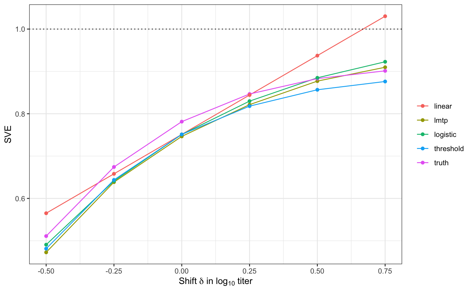

SVE as a function of the shift in log10 titer.

The linear model forces a straight line and soon claims an efficacy above 100%: its “risk” is negative. The misspecified logistic regression keeps predicting benefit from higher titers where there is none, overstating the SVE for positive shifts. The threshold model, like the truth, levels off above the threshold. Plug-in g-computation is only as good as its outcome model. In contrast, lmtp was protected by its density ratio model in Exercise 2.2, even with the misspecified GLM.

2.4.4 Exercise 2.5 💻

Forgetting the design

Re-estimate $\text{SVE}_{0.5}$ with lmtp_tmle() and the Super Learner, without the sampling weights. What happens, and why?

Solution

fit_unwt <- fit_shift(0.5, sl_lib, weights = NULL)
c(
  weighted = 1 - fits_05$super_learner$estimate@x / risk_placebo,
  unweighted = 1 - fit_unwt$estimate@x / risk_placebo,
  truth = true_sve(0.5)$sve
)

  weighted unweighted      truth 
 0.8772560  0.3543930  0.8830436

Without weights, the phase-two sample is treated as representative of all vaccinees, but cases are over-represented about five-fold, so the estimated risk is far too high and the SVE far too low. The estimator must account for the two-phase design.

2.4.5 Exercise 2.6 💻 (stretch)

Positivity and realistic MTPs

Estimate $\text{SVE}_1$, and compare to true_sve(1). Repeat with "SL.glm_threshold" as the outcome model, and compare to its g-computation counterpart from Exercise 2.4. What might explain the result? (Hint: what is the range of vax$S?)
An MTP that respects positivity only shifts people whose shifted titer remains plausible (Hejazi et al. 2021): $d(s, l) = s + \delta$ if $s + \delta \leq u$, and $d(s, l) = s$ otherwise. Implement it with $u$ the 90th percentile of $S$ in the phase-two sample, and re-estimate the SVE curve. How would you interpret this effect?

Solution

# (a) a large shift
range(vax$S)

[1] -0.9046149  2.9612913

c(
  sl = 1 - fit_shift(1, sl_lib)$estimate@x / risk_placebo,
  glm_right = 1 - fit_shift(1, "SL.glm_threshold")$estimate@x / risk_placebo,
  gcomp_right = gcomp_sve(fit_thresh, 1),
  truth = true_sve(1)$sve
)

         sl   glm_right gcomp_right       truth 
  0.9347938   0.9270621   0.8844434   0.9093501

# (b) a positivity-respecting shift, capped at the 90th percentile
u <- quantile(vax$S, 0.9)
shift_capped <- function(delta) {
  function(data, trt) {
    ifelse(data[[trt]] + delta <= u, data[[trt]] + delta, data[[trt]])
  }
}
psi_capped <- sapply(deltas, function(delta) {
  lmtp_tmle(
    data = vax,
    trt = "S",
    outcome = "Y",
    baseline = c("age", "high_risk", "sex"),
    shift = shift_capped(delta),
    outcome_type = "binomial",
    learners_outcome = sl_lib,
    learners_trt = "SL.glm",
    folds = 5,
    weights = 1 / vax$g_R
  )$estimate@x
})
round(
  data.frame(
    delta = deltas,
    capped = 1 - psi_capped / risk_placebo,
    uncapped = sve$lmtp
  ),
  3
)

  delta capped uncapped
1 -0.50  0.473    0.473
2 -0.25  0.639    0.638
3  0.00  0.746    0.746
4  0.25  0.820    0.822
5  0.50  0.872    0.877
6  0.75  0.895    0.910

Shifting titers up by a full $\log_{10}$ unit (10-fold) asks about titers well beyond those observed for many vaccinees. The density ratio becomes extreme and the TML estimate less stable, even with a correct outcome model. Plug-in g-computation with the correct model, by contrast, simply extrapolates its (correct) threshold. This is a near-violation of positivity: the data say little about such large shifts.
The capped MTP answers a different, more realistic question: the effect of raising titers by $\delta$ for those who could plausibly reach the higher titer, leaving others unchanged. Its efficacy gains are smaller, because fewer people are shifted.

2.5 Wrap-up

Both parts targeted causal parameters defined without a model: the ATE $\psi_{0,b}$ of smoking on each CpG, and the SVE, $\text{SVE}_\delta$, under an MTP that shifts antibody titers. We estimated both with machine learning and efficient influence functions.
In both, a linear model gives an appealing shortcut: $\psi_{0,b} = \beta_1$, and $\psi_{0,\delta} - \psi_{0,0} = \beta_1 \delta$. These identities hold only if the linear model is correct; when it is not, the coefficient answers a different (or impossible) question.
A misspecified GLM breaks a plug-in estimator, but not a doubly robust one whose other nuisance is right. Given a library that contains a good model, the Super Learner finds it.
Ideas from classical biomarker analysis still matter: variance moderation for high-dimensional testing (Part 1), and the sampling design (Part 2).
In Part 1, the biomarker was the outcome. In Part 2, it was a mediator of the vaccine’s effect. Decomposing a total effect into pathways through biomarkers (direct and indirect effects) is the subject of causal mediation analysis; see, e.g., the medoutcon package.

Symbol	Meaning
\(L\)	age, high-risk behaviour, sex
\(A\)	vaccine (1) or placebo (0), randomized
\(Y\)	infection by the end of follow-up
\(S\)	immune marker (\(\log_{10}\) antibody titer), a mediator of \(A \to Y\)
\(R\), \(g_{0,R}(Y, L)\)	phase-two sampling indicator, and its known probability \(\P_0(R = 1 \mid Y, L)\)
\(\overline{Q}_{0,Y}(s, l)\)	risk among vaccinees, \(\P_0(Y = 1 \mid S = s, A = 1, L = l)\)
\(g_{0,S}(s \mid l)\)	density of \(S\) given \(A = 1\) and \(L = l\) (generalized propensity score)
\(d(S, L) = S + \delta\)	the modified treatment policy (MTP): an additive shift of \(S\)
\(\psi_{0,\delta}\)	population mean under the MTP, \(\E_0[Y(d(S, L)) \mid A = 1]\)
\(\text{SVE}_\delta\)	\(1 - \psi_{0,\delta} / \P_0(Y = 1 \mid A = 0)\)

2.1 The question

2.2 The data: a simulated trial with a case-cohort design

2.3 The target parameter

2.3.1 Exercise 2.1 ✏️

2.4 Estimation with lmtp

2.4.1 Exercise 2.2 💻

2.4.2 Exercise 2.3 💻

2.4.3 Exercise 2.4 💻

2.4.4 Exercise 2.5 💻

2.4.5 Exercise 2.6 💻 (stretch)

2.5 Wrap-up

2.4 Estimation with `lmtp`