1 Biomarker discovery as causal effect estimation
NoteIn a nutshell
We rebuild the biotmle recipe from its parts. First, we estimate the average treatment effect (ATE) of smoking on methylation at each of many CpG sites by targeted maximum likelihood (TMLE) with machine learning. Then we test all CpGs with variance moderation.
Roadmap: (1) the target parameter, and when a regression coefficient equals it → (2) TMLE by hand, on a synthetic CpG with a known effect → (3) misspecified GLMs, correct GLMs, and Super Learner → (4) the real data, one CpG and then all of them → (5) variance moderation and multiple testing.
NoteNotation for this part
| Symbol | Meaning |
|---|---|
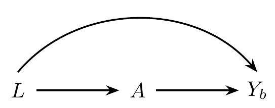
| \(L\) | sex, age, race, and leukocyte proportions |
| \(A\) | smoking status (1 = ever, 0 = never) |
| \(Y_b\), \(b = 1, \ldots, B\) | methylation (M-value) at CpG site \(b\) |
| \(\overline{Q}_{0,b}(A, L)\) | outcome regression for CpG \(b\) |
| \(\psi_{0,b} = \Psi_b(\P_0)\) | ATE of smoking on CpG \(b\) |
| \(H_0(A, L)\) | clever covariate, \(A / g_0(L) - (1 - A) / (1 - g_0(L))\) |
| \(\sigma^2_{n,b}\), \(\tilde{\sigma}^2_{n,b}\) | EIF variance for CpG \(b\), before and after moderation |
1.1 The data: smoking and DNA methylation
Su et al. (2016) measured DNA methylation in whole blood, at roughly 470,000 CpG sites, in 253 people: 172 who had ever smoked and 81 who never had. We use their data to ask: which CpG sites are affected by smoking?
Su, Dan, Xuting Wang, Michelle R Campbell, et al. 2016. “Distinct Epigenetic Effects of Tobacco Smoking in Whole Blood and Among Leukocyte Subtypes.” PLoS ONE 11 (12): e0166486. https://doi.org/10.1371/journal.pone.0166486.
The data on one person are \(O = (L, A, Y) \sim \P_0 \in \mathcal{P}\), where \(\P_0\) is the true, unknown data-generating distribution and \(\mathcal{P}\) is the nonparametric statistical model; we observe \(n\) i.i.d. copies \(O_1, \ldots, O_n\). Here,
-
\(L\) are baseline covariates: sex, age, race, and the estimated proportions of six leukocyte types (
CD8T,CD4T,NK,Bcell,Mono,Gran). Blood cell composition differs by smoking status and strongly affects methylation, so it is a confounder; -
\(A \in \{0, 1\}\) is smoking status (
smoker: 1 = ever, 0 = never); - \(Y = (Y_b : b = 1, \ldots, B)\) are the methylation levels (M-values) at each CpG site \(b\).
To keep computation fast, the file contains \(B = 300\) CpG sites: 150 chosen at random among those flagged by a limma screen in the full data (including four well-known smoking-related CpGs, e.g., cg05575921 in the AHRR gene), and 150 chosen at random among those that were not.
1.2 The target parameter
Let \(g_0(L) = \P_0(A = 1 \mid L)\) be the propensity score and \(\overline{Q}_{0,b}(A, L) = \E_0[Y_b \mid A, L]\) the outcome regression for CpG \(b\). For each CpG, our target is the ATE of smoking on methylation, which (under no unmeasured confounding and positivity) is identified by \[ \psi_{0,b} = \Psi_b(\P_0) = \E_0\big[ \overline{Q}_{0,b}(1, L) - \overline{Q}_{0,b}(0, L) \big]. \] This is a variable importance measure: it ranks CpG sites by how much smoking would change their methylation, without committing to a model for \(\overline{Q}_{0,b}\). Throughout, a subscript \(n\) denotes an estimate (e.g., \(g_n\), \(\overline{Q}_{n,b}\), \(\psi_{n,b}\)).
1.2.1 Exercise 1.1 ✏️
NoteWhen is a regression coefficient the ATE?
The usual approach (as in limma) fits, for each CpG, the working linear model \(\overline{Q}_{0,b}(a, l) = \beta_0 + \beta_1 a + \gamma^\top l\), and tests \(\beta_1 = 0\).
- Suppose this linear model is correct. Show that \(\psi_{0,b} = \beta_1\).
- Now suppose the effect of smoking varies with age, so that the correct model is \(\overline{Q}_{0,b}(a, l) = \beta_0 + \beta_1 a + \beta_2 a \cdot \text{age} + \gamma^\top l\). What is \(\psi_{0,b}\) now? Is \(\beta_1\) still the ATE?
- In (b), what would \(\beta_1\) in the main-terms model of (a) estimate? Is there a study design under which it would still estimate the ATE?
TipSolution
- \(\overline{Q}_{0,b}(1, l) - \overline{Q}_{0,b}(0, l) = (\beta_0 + \beta_1 + \gamma^\top l) - (\beta_0 + \gamma^\top l) = \beta_1\) for every \(l\), so averaging over \(L\) gives \(\psi_{0,b} = \beta_1\).
- Now \(\overline{Q}_{0,b}(1, l) - \overline{Q}_{0,b}(0, l) = \beta_1 + \beta_2 \, \text{age}\), so \(\psi_{0,b} = \beta_1 + \beta_2 \E_0[\text{age}]\). The coefficient \(\beta_1\) is the effect at age 0, which is rarely of scientific interest.
- The main-terms coefficient converges to (roughly) a weighted average of the age-specific effects, with weights proportional to the conditional variance of smoking, \(\V_0(A \mid L)\): people whose smoking status is hard to predict from \(L\) count more. It is not \(\psi_{0,b}\) in general. If \(A\) were randomized (\(A \indep L\)), the main-terms coefficient would be consistent for the ATE even though the model is wrong. Smoking is not randomized, so here we need an estimator whose validity does not hinge on the form of \(\overline{Q}_{0,b}\).
Take-away: \(\psi_{0,b}\) is defined without reference to any model; \(\beta_1\) is \(\psi_{0,b}\) only if the linear model is right (or \(A\) is randomized).
1.3 Efficient estimators: the one-step estimator and TMLE
From the lecture, the efficient influence function (EIF) of \(\psi_{0,b}\) is \[\begin{align*} D_b(O; \P_0) &= H_0(A, L) \big(Y_b - \overline{Q}_{0,b}(A, L)\big) + \overline{Q}_{0,b}(1, L) - \overline{Q}_{0,b}(0, L) - \psi_{0,b} \ , \\ H_0(A, L) &= \frac{A}{g_0(L)} - \frac{1 - A}{1 - g_0(L)} \ . \end{align*}\] Given estimates \(g_n\) and \(\overline{Q}_{n,b}\), the one-step estimator corrects the plug-in estimate by the average of the estimated EIF: \[ \psi^+_{n,b} = \frac{1}{n} \sum_{i = 1}^n \big\{\overline{Q}_{n,b}(1, L_i) - \overline{Q}_{n,b}(0, L_i)\big\} + \frac{1}{n} \sum_{i = 1}^n H_n(A_i, L_i) \big(Y_{b,i} - \overline{Q}_{n,b}(A_i, L_i)\big). \] The correction removes the first-order bias of the plug-in, but the result can fall outside the parameter’s range.
TMLE removes the same bias differently: it updates the initial fit \(\overline{Q}_{n,b}\) to a targeted fit \(\overline{Q}^\star_{n,b}\) chosen so that the average of the estimated EIF is zero, and then plugs it in, \[ \psi^\star_{n,b} = \frac{1}{n} \sum_{i = 1}^n \big\{\overline{Q}^\star_{n,b}(1, L_i) - \overline{Q}^\star_{n,b}(0, L_i)\big\}. \] TMLE is a substitution (plug-in) estimator, \(\psi^\star_{n,b} = \Psi_b(\P^\star_n)\): it is the value of the target parameter at an estimate of the data distribution, so it always respects the parameter’s bounds. Respecting the bounds also tends to make TMLE more stable in finite samples. It shares the one-step estimator’s large-sample properties: it is efficient, its standard error is \(\sqrt{\sigma^2_{n,b} / n}\) with \(\sigma^2_{n,b}\) the empirical variance of the estimated EIF, and it is doubly robust: consistent if either \(g_n\) or \(\overline{Q}_{n,b}\) is consistent.
For a continuous outcome, the update is made on the unit scale, so that the targeted fit respects the observed range of the outcome (Gruber and van der Laan 2010). The helper functions in practical/R/utils.R carry out the parts of each step that are not about TMLE itself:
Gruber, Susan, and Mark J van der Laan. 2010. “A Targeted Maximum Likelihood Estimator of a Causal Effect on a Bounded Continuous Outcome.” The International Journal of Biostatistics 6 (1). https://doi.org/10.2202/1557-4679.1260.
- Scale \(Y_b\) to \([0, 1]\), using its observed range.
-
Helper:
scale_to_unit().
-
Helper:
- Estimate \(g_0\) and (on the unit scale) \(\overline{Q}_{0,b}\). Helpers:
estimate_g()andestimate_Q()fit the nuisance parameters withSuperLearner(), using the library of learners specified.estimate_g()passes its predictions throughbound_propensity(), which truncates predicted probabilities away from 0 and 1, to avoid instability in \(H_n\) (note: truncation does trade a bit of bias for improved variance).bound_precision()keeps the predicted outcomes strictly inside \((0, 1)\), so that their logits (step 4) are finite. - Compute the clever covariate \(H_n(A, L)\), at the observed \(A\) and at \(A = 1\) and \(A = 0\). By hand.
-
Fluctuate: fit the logistic regression \(\operatorname{logit}
\overline{Q}_{n,b}(\epsilon)(A, L) = \operatorname{logit}
\overline{Q}_{n,b}(A, L) + \epsilon H_n(A, L)\), with the initial fit as an offset, giving \(\epsilon_n\). By hand, with
glm(). - Update, \(\overline{Q}^\star_{n,b} = \overline{Q}_{n,b}(\epsilon_n)\), and plug in. Fitting \(\epsilon\) by maximum likelihood makes the average of the EIF zero: TMLE solves the EIF estimating equation. By hand.
- Compute the EIF at the targeted fit for the standard error, and scale back to the original units (multiplying by the range of \(Y_b\), as
scale_from_unit()does). By hand.
tmle_ate() wraps all six steps; we use it once we have done them by hand.
1.3.1 A synthetic CpG with a known effect
Before turning to the real data, we try TMLE on a synthetic CpG for which we know the true causal effect. In sim_cpg(), \(L = (\text{bmi}_z,
\text{sex})\), where \(\text{bmi}_z\) is a standardized body-mass index (a \(z\)-score), and \[\begin{align*}
g_0(L) &= \operatorname{expit}(-1 + 0.7\, \text{bmi}_z^2 + 0.4\, \text{sex}) \ , \\
\overline{Q}_0(A, L) &= 0.5 - A + 0.3\, \text{bmi}_z + 0.8\, \text{bmi}_z^2 +
0.2\, \text{sex} \ ,
\end{align*}\] so the true ATE is \(\psi_0 = -1\). A main-terms GLM in \((A, \text{bmi}_z,
\text{sex})\) omits the confounding through \(\text{bmi}_z^2\) and is misspecified; the learner SL.glm_correct (in practical/R/learners.R) adds \(\text{bmi}_z^2\) and is correctly specified.
1.3.2 Exercise 1.2 💻
NoteTMLE by hand
Complete the steps below to compute the TMLE of the ATE of the synthetic CpG, with correctly specified GLMs for both \(g_0\) and \(\overline{Q}_0\). Check that the average of the estimated EIF at the targeted fit is (numerically) zero.
# 1. scale the outcome to [0, 1]
y_range <- range(cpg_sim$Y)
y_s <- scale_to_unit(cpg_sim$Y, y_range)

# 2. initial estimates of g_0 and of Q_0 (on the unit scale)
g_n <- estimate_g(a_sim, l_sim, g_lib = "SL.glm_correct")
Q_n <- estimate_Q(y_s, a_sim, l_sim, q_lib = ___)
QA <- bound_precision(Q_n$QA)
Q1 <- bound_precision(Q_n$Q1)
Q0 <- bound_precision(Q_n$Q0)

# 3. the clever covariate, at the observed A, at A = 1, and at A = 0
H_A <- ___
H_1 <- 1 / g_n
H_0 <- -1 / (1 - g_n)

# 4. fluctuate: logistic regression on H_A, with the initial fit as offset
fluc <- glm(y_s ~ -1 + H_A + offset(qlogis(QA)), family = quasibinomial())
eps <- coef(fluc)

# 5. update the initial fit, and plug in
Q1_star <- plogis(qlogis(Q1) + eps * ___)
Q0_star <- plogis(qlogis(Q0) + eps * ___)
QA_star <- plogis(qlogis(QA) + eps * H_A)
psi_s <- mean(___)

# 6. the EIF at the targeted fit, and the estimate on the original scale
eif <- diff(y_range) * (H_A * (y_s - QA_star) + Q1_star - Q0_star - psi_s)
c(
  psi = diff(y_range) * psi_s,
  se = sd(eif) / sqrt(nrow(cpg_sim)),
  mean_eif = mean(eif)
)
TipSolution
# 1. scale the outcome to [0, 1]
y_range <- range(cpg_sim$Y)
y_s <- scale_to_unit(cpg_sim$Y, y_range)

# 2. initial estimates of g_0 and of Q_0 (on the unit scale)
g_n <- estimate_g(a_sim, l_sim, g_lib = "SL.glm_correct")
Q_n <- estimate_Q(y_s, a_sim, l_sim, q_lib = "SL.glm_correct")
QA <- bound_precision(Q_n$QA)
Q1 <- bound_precision(Q_n$Q1)
Q0 <- bound_precision(Q_n$Q0)

# 3. the clever covariate, at the observed A, at A = 1, and at A = 0
H_A <- a_sim / g_n - (1 - a_sim) / (1 - g_n)
H_1 <- 1 / g_n
H_0 <- -1 / (1 - g_n)

# 4. fluctuate: logistic regression on H_A, with the initial fit as offset
fluc <- glm(y_s ~ -1 + H_A + offset(qlogis(QA)), family = quasibinomial())
eps <- coef(fluc)

# 5. update the initial fit, and plug in
Q1_star <- plogis(qlogis(Q1) + eps * H_1)
Q0_star <- plogis(qlogis(Q0) + eps * H_0)
QA_star <- plogis(qlogis(QA) + eps * H_A)
psi_s <- mean(Q1_star - Q0_star)

# 6. the EIF at the targeted fit, and the estimate on the original scale
eif <- diff(y_range) * (H_A * (y_s - QA_star) + Q1_star - Q0_star - psi_s)
c(
  psi = diff(y_range) * psi_s,
  se = sd(eif) / sqrt(nrow(cpg_sim)),
  mean_eif = mean(eif)
)
psi se mean_eif
-1.003542e+00 3.256159e-02 4.871104e-17 [1] -1.002366With correctly specified GLMs, the initial plug-in estimate is already close to \(-1\), and the targeting step barely moves it (\(\epsilon_n\) is small). The mean of the EIF at the targeted fit is zero up to numerical error: that is what the fluctuation step is for.
As a check, tmle_ate(), given the propensity score estimates and a library for \(\overline{Q}_0\), reproduces the computation above:
1.3.3 Exercise 1.3 💻
NoteMisspecified GLMs, correct GLMs, and Super Learner
- Using
estimate_g()andtmle_ate(), estimate the ATE of the synthetic CpG with all four combinations of misspecified ("SL.glm") and correct ("SL.glm_correct") GLMs for \(g_0\) and \(\overline{Q}_0\). Before running the code: which combinations do you expect to give a (nearly) unbiased estimate? How does the main-terms regression coefficient compare? - In practice, we don’t know which GLM is correct. Re-estimate the ATE with Super Learner for both nuisance parameters, using the library below, which includes the correct GLM among other candidates: the main-terms GLM, lasso and ridge regression (
glmnet), MARS (earth), and a generalized additive model (gam). Which learners does the Super Learner weight most heavily?
# (a) GLMs
g_wrong <- estimate_g(a_sim, l_sim, "SL.glm")
g_right <- estimate_g(a_sim, l_sim, ___)
rbind(
  both_wrong = tmle_ate(cpg_sim$Y, a_sim, l_sim, g_wrong, "SL.glm"),
  both_right = tmle_ate(cpg_sim$Y, a_sim, l_sim, g_right, "SL.glm_correct"),
  q_wrong_g_right = tmle_ate(___),
  q_right_g_wrong = tmle_ate(___)
)
coef(lm(Y ~ A + bmi_z + sex, data = cpg_sim))[["A"]]

# (b) Super Learner
sl_lib <- c(
  "SL.mean",
  "SL.glm",
  "SL.glm_correct",
  "SL.glmnet",
  "SL.ridge",
  "SL.earth",
  "SL.gam"
)
g_sl <- estimate_g(___)
tmle_ate(cpg_sim$Y, a_sim, l_sim, g_sl, ___)
round(estimate_Q(cpg_sim$Y, a_sim, l_sim, sl_lib)$coef, 2)
TipSolution
# (a) GLMs
g_wrong <- estimate_g(a_sim, l_sim, "SL.glm")
g_right <- estimate_g(a_sim, l_sim, "SL.glm_correct")
rbind(
  both_wrong = tmle_ate(cpg_sim$Y, a_sim, l_sim, g_wrong, "SL.glm"),
  both_right = tmle_ate(cpg_sim$Y, a_sim, l_sim, g_right, "SL.glm_correct"),
  q_wrong_g_right = tmle_ate(cpg_sim$Y, a_sim, l_sim, g_right, "SL.glm"),
  q_right_g_wrong = tmle_ate(cpg_sim$Y, a_sim, l_sim, g_wrong, "SL.glm_correct")
)
psi se mean_eif
both_wrong -0.1706585 0.05822168 -2.138787e-13
both_right -1.0035424 0.03256159 4.871104e-17
q_wrong_g_right -1.0428640 0.05916187 4.183320e-16
q_right_g_wrong -1.0023752 0.02211830 -1.510482e-12[1] -0.1762296 psi se mean_eif
-1.004047e+00 2.831007e-02 -1.483626e-11 SL.mean_All SL.glm_All SL.glm_correct_All SL.glmnet_All
0.00 0.00 0.99 0.00
SL.ridge_All SL.earth_All SL.gam_All
0.00 0.00 0.01 - By double robustness, every combination except “both wrong” is consistent. With both GLMs misspecified, the estimate is far from \(-1\): the omitted \(\text{bmi}_z^2\) confounds the comparison, just as it does for the main-terms regression coefficient. With only \(g_n\) correct, the estimate is nearly unbiased but noisier: the targeting step then does all the work, through the weights \(H_n\), which are large for some people.
- The Super Learner puts most of its weight on
SL.glm_correct: by cross-validation, it finds the correctly specified GLM among the candidates and recovers the truth. Had no candidate been correct, it would still pick the best-predicting combination, and double robustness only needs one of \(g_n\) and \(\overline{Q}_n\) to be (close to) right.
1.4 Back to the real data
For the methylation data, we do not know the correct model, so we rely on the Super Learner. We drop SL.glm_correct, which is specific to the synthetic CpG, and SL.gam, whose backfitting fails on the nearly collinear cell-type proportions (which sum to about one).
1.4.1 Exercise 1.4 💻
NoteThe linear model, and AHRR
- Fit the working linear model of Exercise 1.1(a) to each CpG, collecting \(\beta_{n,1}\), its standard error, and its \(t\)-statistic.
- Notice that \(g_0(L)\) does not depend on \(b\): estimate it once, with the Super Learner.
- Estimate the ATE of smoking on
cg05575921(AHRR) by TMLE, with the Super Learner and withq_lib = "SL.glm". Compare both to the linear model’s \(\beta_{n,1}\). Why is the"SL.glm"version so close to it?
# (a) the linear-model baseline
lm_one <- function(cpg) {
  fit <- lm(reformulate(c("smoker", covars), response = cpg), data = methy)
  coef(summary(fit))[___, c("Estimate", "Std. Error", "t value")]
}
lm_res <- t(sapply(cpgs, lm_one))
head(lm_res[order(-abs(lm_res[, "t value"])), ])

# (b) the propensity score, once
real_lib <- setdiff(sl_lib, c("SL.glm_correct", "SL.gam"))
g_n <- estimate_g(___, ___, real_lib)

# (c) one CpG
rbind(sl = tmle_ate(methy$cg05575921, A, L, g_n, real_lib), glm = tmle_ate(___))
lm_res["cg05575921", ]
TipSolution
             Estimate Std. Error    t value
cg05575921 -1.7162551 0.05852813 -29.323592
cg21566642 -0.7905914 0.04415236 -17.905982
cg03636183 -0.6788992 0.05405966 -12.558333
cg19859270 -0.6294083 0.06298618  -9.992800
cg08709672 -0.2169516 0.02496367  -8.690693
cg19614919 -0.3696805 0.04559097 -8.108634 Min. 1st Qu. Median Mean 3rd Qu. Max.
0.4426 0.6065 0.6850 0.6798 0.7586 0.8935 psi se mean_eif
sl -1.749647 0.04974591 -5.693329e-13
glm -1.739676 0.04975121 -8.631651e-13 Estimate Std. Error t value
-1.71625514 0.05852813 -29.32359214 The AHRR CpG is at the top of the linear-model ranking, as in large epigenome-wide studies of smoking (Joehanes et al. 2016). With \(\overline{Q}_{n,b}\) from the main-terms GLM, the initial plug-in estimate \(\frac{1}{n}\sum_i \{\overline{Q}_{n,b}(1, L_i) - \overline{Q}_{n,b}(0, L_i)\}\) is exactly \(\beta_{n,1}\) (Exercise 1.1a); the targeting step then moves it only as much as the data, through \(g_n\), indicate that the linear model is misspecified. When the linear model fits well, that step is small.
Joehanes, Roby, Allan C. Just, Riccardo E. Marioni, et al. 2016. “Epigenetic Signatures of Cigarette Smoking.” Circulation: Cardiovascular Genetics 9 (5): 436–47. https://doi.org/10.1161/CIRCGENETICS.116.001506.
1.4.2 Exercise 1.5 💻
NoteAll CpGs
Apply tmle_ate(), with the Super Learner, to every CpG. (This takes a minute or two.) Since we will need the variance of the EIF, \(\sigma^2_{n,b}\), recover it from the standard error.
TipSolution
                  psi         se      mean_eif        s2
cg05575921 -1.7434290 0.04970326 -7.168693e-13 0.6250148
cg21566642 -0.8296899 0.03834594 -4.300469e-17 0.3720139
cg03636183 -0.7174997 0.04960191 -7.159714e-10 0.6224684
cg19859270 -0.6361967 0.05935419 -5.446029e-11 0.8912987
cg13591352  0.2373700 0.03620747  2.863168e-13 0.3316781
cg04255770 -0.3362369 0.05061981 -3.911896e-12 0.6482784[1] 0.99800981.5 Variance moderation
With many biomarkers and few samples, some \(\sigma^2_{n,b}\) will be tiny by chance, producing large test statistics for small effects. The moderated \(t\)-statistic of Smyth (2004) borrows strength across biomarkers by shrinking each variance towards a common value, \[
\tilde{\sigma}^2_{n,b} = \frac{d_b \, \sigma^2_{n,b} + d_0 \, s_0^2}{d_b +
d_0}, \qquad
\tilde{t}_{n,b} = \frac{\psi^\star_{n,b}}{\sqrt{\tilde{\sigma}^2_{n,b} / n}},
\] where \(d_b\) are the degrees of freedom of \(\sigma^2_{n,b}\), and the prior degrees of freedom \(d_0\) and prior variance \(s_0^2\) are estimated from all \(B\) variances by empirical Bayes. \(\tilde{t}_{n,b}\) is compared to a \(t\)-distribution with \(d_b + d_0\) degrees of freedom. biotmle’s key observation (Hejazi et al. 2023) is that nothing in this recipe requires \(\sigma^2_{n,b}\) to come from a linear model: it can be the variance of the EIF.
Smyth, Gordon K. 2004. “Linear Models and Empirical Bayes Methods for Assessing Differential Expression in Microarray Experiments.” Statistical Applications in Genetics and Molecular Biology 3 (1): 1–25. https://doi.org/10.2202/1544-6115.1027.
The function moderate(s2, df) (in practical/R/moderate.R) implements this shrinkage, reproducing limma::squeezeVar(); it returns s2_tilde, d0, and s0_2.
1.5.1 Exercise 1.6 ✏️
NoteHow much shrinkage?
- What does \(\tilde{\sigma}^2_{n,b}\) become as \(d_0 \to 0\)? As \(d_0 \to \infty\)?
- Here, \(d_b = n - 1 = 252\). Suppose empirical Bayes estimates \(d_0 \approx 5\). What fraction of \(\tilde{\sigma}^2_{n,b}\) comes from the prior? When would moderation matter more?
- Why might the EIF-based variance \(\sigma^2_{n,b}\) be more erratic than the linear model’s residual variance, making moderation especially valuable?
TipSolution
- As \(d_0 \to 0\), \(\tilde{\sigma}^2_{n,b} \to \sigma^2_{n,b}\): no moderation, an ordinary \(t\)-statistic. As \(d_0 \to \infty\), \(\tilde{\sigma}^2_{n,b} \to s_0^2\): every biomarker shares one variance, and tests rank biomarkers by effect size alone.
- The weight on the prior is \(d_0 / (d_b + d_0) = 5 / 257 \approx 2\%\), so moderation barely changes anything at \(n = 253\). It matters when \(n\) is small (say, \(n = 10\)–\(30\), as in many expression studies), where \(d_b\) is comparable to \(d_0\).
- The EIF involves \(H_n\), i.e., \(1 / g_n(L)\), which can be large for a few people (as in Exercise 1.3a). It also involves flexible \(\overline{Q}_{n,b}\) fits, whose residuals vary across CpGs. The EIF variance estimator is only asymptotically valid: in small samples, it can be too small for some CpGs (false positives) and too large for others. Shrinkage stabilizes it without giving up model-agnostic inference.
1.5.2 Exercise 1.7 💻
NoteModerated tests and multiple testing
- Moderate the EIF variances, compute moderated \(t\)-statistics and \(p\)-values, and adjust for multiple testing with the Benjamini–Hochberg procedure (Benjamini and Hochberg 1995).
-
(Optional.) Applying the same function to the linear models’ residual variances gives
limma’s moderated \(t\)-statistic. Do so, and compare the two lists of discoveries.
Benjamini, Yoav, and Yosef Hochberg. 1995. “Controlling the False Discovery Rate: A Practical and Powerful Approach to Multiple Testing.” Journal of the Royal Statistical Society: Series B (Methodological) 57 (1): 289–300. https://doi.org/10.1111/j.2517-6161.1995.tb02031.x.
# (a) biotmle: moderate the EIF variances
mod_eif <- moderate(tmle_res[, "s2"], df = ___)
t_eif <- tmle_res[, "psi"] / sqrt(___ / n)
p_eif <- 2 * pt(-abs(t_eif), df = n - 1 + mod_eif$d0)
q_eif <- p.adjust(p_eif, method = "BH")

# (b) limma: moderate the residual variances of the linear models
df_lm <- n - length(covars) - 2
...
TipSolution
       d0      s0_2
4.3651262 0.3660632
# (b) limma: moderate the residual variances of the linear models
df_lm <- n - length(covars) - 2
sigma_lm <- sapply(cpgs, function(cpg) {
sigma(lm(reformulate(c("smoker", covars), response = cpg), data = methy))
})
unscaled_se <- lm_res[, "Std. Error"] / sigma_lm
mod_lm <- moderate(sigma_lm^2, df = df_lm)
t_lm <- lm_res[, "Estimate"] / (unscaled_se * sqrt(mod_lm$s2_tilde))
p_lm <- 2 * pt(-abs(t_lm), df = df_lm + mod_lm$d0)
q_lm <- p.adjust(p_lm, method = "BH")
table(biotmle = q_eif < 0.05, limma = q_lm < 0.05) limma
biotmle FALSE TRUE
FALSE 127 0
TRUE 8 165res <- data.frame(cpg = cpgs, psi = tmle_res[, "psi"], q = q_eif)
ggplot(res, aes(psi, -log10(q), colour = q < 0.05)) +
geom_point(alpha = 0.7) +
geom_hline(yintercept = -log10(0.05), linetype = "dashed") +
geom_text(
data = subset(res, cpg == "cg05575921"),
aes(label = "AHRR"),
nudge_x = 0.15,
colour = "black"
) +
labs(
x = "Estimated ATE of smoking (M-value scale)",
y = expression(-log[10](q)),
colour = "FDR < 5%"
) +
theme_bw()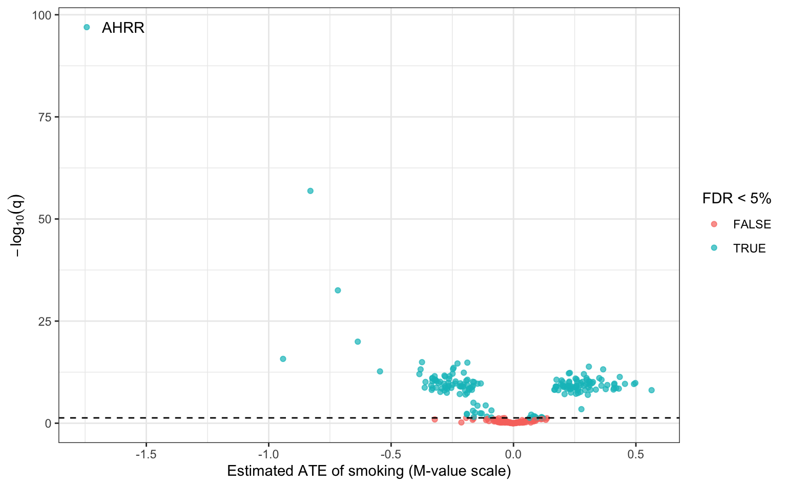
The two procedures largely agree here: the linear model seems a reasonable working model for most CpGs, and \(n\) is large enough that moderation is mild. Where they disagree is precisely where the linear model’s assumptions are doing work that the data cannot verify.
1.5.3 Exercise 1.8 ✏️ (stretch)
NoteTwo-stage analyses
These 300 CpGs were themselves selected: half passed a screen applied to all 472,678 CpGs measured. The published analysis (Hejazi et al. 2023) screens with limma, runs biotmle on the 2,537 CpGs that pass, and adjusts \(p\)-values as if all 472,678 had been tested (setting \(p = 1\) for those screened out) (Tuglus and van der Laan 2009). Why is adjusting only over the CpGs that pass the screen not enough?
Tuglus, Catherine, and Mark J van der Laan. 2009. “Modified FDR Controlling Procedure for Multi-Stage Analyses.” Statistical Applications in Genetics and Molecular Biology 8 (1). https://doi.org/10.2202/1544-6115.1397.
Hejazi, Nima S, Philippe Boileau, Mark J van der Laan, and Alan E Hubbard. 2023. “A Generalization of Moderated Statistics to Data Adaptive Semiparametric Estimation in High-Dimensional Biology.” Statistical Methods in Medical Research 32 (3): 539–54. https://doi.org/10.1177/09622802221146313.
TipSolution
The screen used the same data, and kept CpGs because their association with smoking looked strong. Testing only the survivors, and correcting only for their number, ignores the selection: the error rate would be computed over a set of hypotheses chosen to look significant. Counting every CpG measured in the multiplicity correction accounts for the first stage.