Cross-Trial Causal Comparison of Treatment Regimens Without a Common Comparator: A Case Study of MDR/RR-TB

April 21, 2026
MDR/RR-TB and HIV
- Drug-resistant TB (MDR/RR-TB) remains a major global cause of preventable morbidity and mortality.
- People living with HIV (PLHIV) face substantially higher TB risk, and TB is a leading cause of death among PLHIV.
- Clinicians and programs need evidence to choose among new all-oral regimens.
New hope: shorter, all-oral MDR/RR-TB regimens
Recent trials introduced short-course, all-oral regimens:
- TB-PRACTECAL (Nyang’wa et al., 2022, 2024)
- 6-month regimen: 6BPaLM (Bedaquiline + Pretomanid + Linezolid + Moxifloxacin)
- Non-inferior vs standard care
- endTB (Guglielmetti et al., 2025)
- 9-month regimens: 9BLMZ, 9BCLLfxZ, 9BDLLfxZ
- Non-inferior vs standard care
Standard care in each study was
- TB-PRACTECAL: 9–12 or 18–20 month all-oral regimens (region-specific)
- endTB: 18–20 month all-oral regimens (region-specific)
The decision problem: no head-to-head evidence
- WHO guidelines recommend multiple all-oral MDR/RR-TB regimens; shorter regimens are appealing for feasibility and adherence.
- However, comparative evidence between 6-month and 9-month regimens is limited, and certainty of evidence is often low.
Question: Is 6BPaLM truly preferable to 9-month regimens from endTB?
What data do we have: two high-quality RCTs
We have individual patient data (IPD) from two non-inferiority RCTs:
| Feature | TB-PRACTECAL | endTB |
|---|---|---|
| Duration | 6-month regimens | 9-month regimens |
| Standard care | 9–12 or 18–20 month all-oral regimens (region-specific) | 18–20 month all-oral regimens (region-specific) |
| Study regions | Uzbekistan, Belarus, South Africa | Georgia, India, Kazakhstan, Lesotho, Pakistan, Peru, South Africa |
| Follow-up time | At least 72 weeks | At least 73 weeks |
- No head-to-head regimen comparison (no common arm)
- Heterogeneous standard care (region/time-specific)
- Population and setting differences across trial regions (affects transportability)
Because a new head-to-head RCT is unlikely in the near term, we need to make the best possible use of existing evidence through cross-trial data fusion.
Aim and Approaches
Primary aim: Compare the efficacy of 6BPaLM versus endTB regimen (9BLMZ, 9BCLLfxZ, 9BDLLfxZ).
Approaches:
- Meta-analytic approach: apply meta analysis to estimate direct contrasts.
- Target trial emulation approach: use target trial emulation framework (Hernán & Robins, 2016), then analyze as an observational study.
- Pooled-IPD “direct” strategy: Pool individual patient data (IPD) from both trials and estimate the direct head-to-head contrast between the two treatments of intests.
- Pooled-IPD “indirect” strategy: Pool IPD from both trials and estimate the indirect contrast between treatments despite non-common comparator (standard care).
Related Literature and Contribution
- Transportability
- Prior work studies how to transport causal effects from multiple randomized trials to a new target population where experimental data may not be available (Dahabreh et al., 2020; Dahabreh and Hernán, 2019).
- The core assumption of these methods lies in addressing the covariate distribution shift between the “experiment” and “target” groups.
- Common trial structure assumption
Much of the causal transportability and IPD meta-analysis literature considers settings where trials evaluate the same treatment set or comparator, which simplifies pooling or transport of treatment effects (e.g., (Dahabreh et al., 2020)).
Our setting and contribution
- We define a target population as the union of participants from endTB and TB-PRACTECAL and focus on cross-trial causal comparison.
- We compare four strategies by combining ideas from transportability, target trial emulation, and IPD meta-analysis In particular, standard cares comparison can be solved in our framework by appropriately adjusting for differences.
Data Structure and Notation
Populations:
- \(S \in \{1,2\}\): trial indicator
- \(S=1\): endTB
- \(S=2\): TB-PRACTECAL
- \(\Omega\): target population of interest
Variables:
- \(A \in \mathcal{A}\): treatment received
- \(a\): 6BPaLM
- \(b\): endTB regimen (9BLMZ, 9BCLLfxZ, 9BDLLfxZ)
- \(c_s\): standard care in trial (S=s)
- \(Y\): outcome (e.g., unfavorable outcome by end of follow-up)
- \(L\): baseline covariates (measured pre-treatment)
Overview of four data fusion methods
Target population of interest \(\Omega\): consisting of individuals at risk of TB recurrence in countries hosting enrollment sites for either the endTB or TB-PRACTECAL trials .
\(\Omega = \Omega_{\text{TB-PRACTECAL}} \cup \Omega_{\text{endTB}}\)
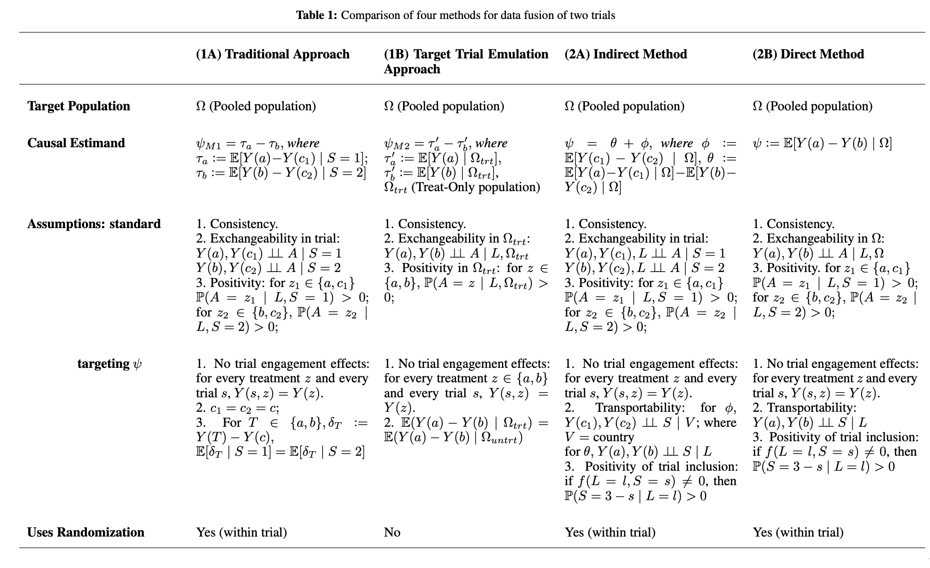
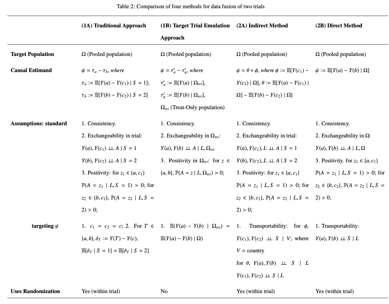
| Method | Key Idea | Target Population |
|---|---|---|
| (1) Traditional Approach | Compare each treatment to control in each trial, then take the difference of the estimates (possibly with weighting) | \(\Omega\) (Pooled) |
| (2) Target Trial Emulation Approach | Combine treatment arms by developing target trial protocols, analyze as an observational study | \(\Omega\) (Pooled) |
| (3) Direct Method | Estimate direct contrast by pooling data and adjusting for trial specific differences | \(\Omega\) (Pooled) |
| (4) Indirect Method | Decompose contrast into treatment effect difference + control effect difference | \(\Omega\) (Pooled) |
All methods aim to estimate the casual estimand: \[\psi(a, b) = \mathbb{E}[Y(a) - Y(b) \mid \Omega].\]
Method 1: Traditional approach
The Core Idea: Use randomization within each trial, then take the difference of the estimated effects.
What the traditional approach does:
- Analyze each trial separately: Calculate within trial effect with data from TB-PRACTECAL and endTB separately.
- Compare the two results: Take the difference between the two trial-specific effects.
Strength: Uses within trial randomization
Limitation: Assumes negligible differences in standard-care efficacy between endTB and TB-PRACTECAL, as achieved by having a common comparator.
This directly reflects the common comparator: \(\mathbb{E}[Y(c_1) - Y(c_2) \mid \Omega] = 0\)
Method 1: Traditional Approach — Estimand
Estimand: Compare trial-specific treatment-vs-control contrasts, then take the difference.
Define trial-specific causal effects: \[ \tau_a := \mathbb{E}[Y(a) - Y(c_1) \mid S=1], \qquad \tau_b := \mathbb{E}[Y(b) - Y(c_2) \mid S=2] \]
The traditional indirect comparison estimand is \(\tau_a - \tau_b.\)
Recall the target causal estimand is \(\psi(a,b) = \mathbb{E}[Y(a)-Y(b)\mid\Omega]\), which decomposes as \[ \psi = \underbrace{\mathbb{E}[Y(a)-Y(c_1)\mid\Omega] - \mathbb{E}[Y(b)-Y(c_2)\mid\Omega]}_{\theta} + \underbrace{\mathbb{E}[Y(c_1)-Y(c_2)\mid\Omega]}_{\phi}. \]
The traditional method targets \(\theta\), not \(\psi\) — unless \(\phi = 0\).
Method 1: Identification Assumptions
| Label | Assumption |
|---|---|
| M1.1 | Consistency: \(Y = Y(z)\,\mathbf{1}(A=z)\) for all \(z\in\{a,b,c_1,c_2\}\) |
| M1.2 | Exchangeability within each trial: \(Y(a),Y(c_1)\perp\!\!\!\perp A\mid S=1\); \(Y(b),Y(c_2)\perp\!\!\!\perp A\mid S=2\) |
| M1.3 | Positivity: \(P(A=z\mid S=s)>0\) for each arm \(z\) in trial \(s\) |
| M1.4 | No trial engagement effects: \(Y(s,z)=Y(z)\) — potential outcomes do not depend on trial membership |
| M1.5 | Harmonized control: \(c_1=c_2=c\), or weakly, \(\phi := \mathbb{E}[Y(c_1)-Y(c_2)\mid\Omega]=0\) |
| M1.6 | Homogeneity of control-relative effects: \(\mathbb{E}[\delta_a\mid S=1]=\mathbb{E}[\delta_a\mid S=2]\), \(\mathbb{E}[\delta_b\mid S=1]=\mathbb{E}[\delta_b\mid S=2]\), where \(\delta_t:=Y(t)-Y(c_t)\) |
M1.1–M1.4 guarantee identification of each trial-specific ATE by randomization. M1.5–M1.6 are the strong additional conditions required to recover \(\psi\): they are not directly testable from the observed two-trial data.
Method 1: Identification Theorem and Proof Sketch
Theorem 1. Under M1.1–M1.4, \(\tau_a - \tau_b\) is identified: \[ \tau_a = \mathbb{E}[Y\mid A=a, S=1] - \mathbb{E}[Y\mid A=c_1, S=1], \] and analogously for \(\tau_b\). Under M1.5–M1.6, \(\tau_a - \tau_b = \psi(a,b).\)
Proof sketch. M1.5 implies \(\phi=0\), so \(\psi = \theta\). For \(\theta\), apply the law of total expectation over \(\Omega = \Omega_1\cup\Omega_2\): \[ \theta = \mathbb{E}[Y(a)-Y(c_1)\mid\Omega] - \mathbb{E}[Y(b)-Y(c_2)\mid\Omega] \overset{\text{M1.6}}{=} \tau_a - \tau_b. \qquad\square \] M1.6 is the critical step: it requires the mean control-relative effect for each active treatment to be invariant across trial populations — a strong, scale-dependent restriction with no nonparametric test from the observed data.
Method 1: Estimation and Inference
Within each trial, \(\tau_a\) and \(\tau_b\) can be estimated via:
IPW: \(\hat{\tau}_a^{\text{IPW}} = \mathbb{P}_{\Omega,n}\!\left[\dfrac{\mathbf{1}(A=a,S=1)}{P(A=a\mid S=1)}Y - \dfrac{\mathbf{1}(A=c_1,S=1)}{P(A=c_1\mid S=1)}Y\right]\)
G-computation: \(\hat{\tau}_a^{G} = \hat{\mu}_1(a) - \hat{\mu}_1(c_1)\)
EIF-based (one-step/doubly robust): augments IPW with outcome regression; consistent if either nuisance model is correctly specified.
Because the two trials are independent, asymptotic normality follows directly: \[ \sqrt{n}\bigl[(\hat{\tau}_a - \hat{\tau}_b) - (\tau_a-\tau_b)\bigr] \xrightarrow{d} \mathcal{N}\!\left(0,\,\sigma_a^2 + \sigma_b^2\right). \] Variance estimation: sandwich estimators or nonparametric bootstrap applied independently within each trial.
Method 2: Target Trial Emulation Approach
Core idea: Construct an emulated trial by pooling treated arms across trials and analyzing the data as an observational study, following a target trial emulation protocol while ignoring standard-care arms.
Motivation: Conducting a new head-to-head randomized trial is often infeasible. By discarding control arms and comparing treated groups directly, we extract maximal information from existing trials under explicit causal assumptions.
What this approach does:
Specify a target trial protocol (eligibility, treatment strategies, outcome, follow-up). <!–
Restrict data to treated participants. –>
Pool treated arms across trials to form a single analytic dataset.
Adjust for baseline covariates to control for possible confounding.
Method 2: Target Trial Emulation Approach
Identification
Exchangeability is assumed conditional on measured covariates.
Randomization is no longer used once control arms are discarded.
Limitation
Because control arms are ignored, identification relies entirely on covariate adjustment rather than randomization.
Lower sample size due to discarding control arms.
Method 2: Target Trial Emulation — Setup
Core idea: Reframe cross-trial evidence synthesis as the emulation of a hypothetical head-to-head RCT (Hernán & Robins, 2016). Pool the treated arms across trials and analyze the combined dataset as an observational study.
Let \(\Omega_{\text{trt}}\) denote the subpopulation of treated participants. The pooled treated dataset is \[ \mathcal{O}^{\text{pool}}_{\text{trt}} = \{(Y_i, A_i, L_i, S_i) : A_i \in \{a, b\},\; i \in \Omega_{\text{trt}}\}. \]
Target estimand in this approach: \[ \tau'_a - \tau'_b, \quad \text{where}\quad \tau'_a := \mathbb{E}[Y(a)\mid\Omega_{\text{trt}}],\quad \tau'_b := \mathbb{E}[Y(b)\mid\Omega_{\text{trt}}]. \]
Key structural consequence: Once treated arms are pooled, treatment assignment between \(a\) and \(b\) is confounded with trial membership — within-trial randomization no longer applies. The pooled dataset must be analyzed as an observational study.
Method 2: Identification Assumptions
| Label | Assumption |
|---|---|
| M2.1 | Consistency |
| M2.2 | Conditional exchangeability in \(\Omega_{\text{trt}}\): \(Y(a),Y(b)\perp\!\!\!\perp A\mid L,\,\Omega_{\text{trt}}\) |
| M2.3 | Positivity in \(\Omega_{\text{trt}}\): \(P(A=z\mid L,\,\Omega_{\text{trt}})>0\) for \(z\in\{a,b\}\) |
| M2.4 | No trial engagement effects: \(Y(s,z)=Y(z)\) |
| M2.5 | Homogeneity across treatment-uptake subgroups: \(\mathbb{E}[Y(a)-Y(b)\mid\Omega_{\text{trt}}]=\mathbb{E}[Y(a)-Y(b)\mid\Omega]\) |
Theorem 2. Under M2.1–M2.4, \(\tau'_a - \tau'_b\) is identified from \(\mathcal{O}^{\text{pool}}_{\text{trt}}\): \[ \tau'_a - \tau'_b = \mathbb{E}[\mathbb{E}(Y\mid A=a, L, \Omega_{\text{trt}})] - \mathbb{E}[\mathbb{E}(Y\mid A=b, L, \Omega_{\text{trt}})]. \] Under M2.4–M2.5, \(\tau'_a - \tau'_b = \psi(a,b).\)
Method 2: Assumptions — Closer Look
M2.2 (Exchangeability) requires that, conditional on \(L\), treatment assignment is independent of potential outcomes within \(\Omega_{\text{trt}}\). This is the standard unconfoundedness condition for observational data — not guaranteed by randomization.
M2.5 (Homogeneity) requires that the average treatment effect is the same in the treated and untreated subpopulations:
\[ \begin{align*} \mathbb{E}[Y(a) - Y(b)\mid \Omega] &= \mathbb{E}[Y(a) - Y(b)\mid \Omega_{\mathrm{trt}}] \mathbb{P}(\Omega_{\mathrm{trt}})+ \mathbb{E}[Y(a) - Y(b)\mid \Omega_{\mathrm{untrt}}] \mathbb{P}(\Omega_{\mathrm{untrt}}) \\ &=\mathbb{E}[Y(a) - Y(b)\mid \Omega_{\mathrm{trt}}] \left[ \mathbb{P}(\Omega_{\mathrm{trt}}) + \mathbb{P}(\Omega_{\mathrm{untrt}})\right]\\ &=\mathbb{E}[Y(a) - Y(b)\mid \Omega_{\mathrm{trt}}], \end{align*} \]
where the second equation requires that \(\mathbb{E}[Y(a) - Y(b)\mid \Omega_{\mathrm{trt}}] = \mathbb{E}[Y(a) - Y(b)\mid \Omega_{\mathrm{untrt}}]\).
Thus, identifying the full-population effect using only treated individuals requires \[ \mathbb{E}[Y(a) - Y(b)\mid \Omega_{\mathrm{trt}}] = \mathbb{E}[Y(a) - Y(b)\mid \Omega_{\mathrm{untrt}}], \] i.e., equality of causal effects across treatment-uptake groups.
Methods 3 and 4: Direct and Indirect Approaches
Merge the data from TB-PRACTECAL and endTB, and extend inferences from trial participants to the target population of interest (i.e., \(\Omega\)).
Due to \(\Omega = \Omega_{\text{TB-PRACTECAL}} \cup \Omega_{\text{endTB}},\) we
- use law of total expectation to decompose \(\Omega\) into each trial’s population;
- apply transportability to answer questions such as: “What would be the average treatment effect if the endTB participants had received the TB-PRACTECAL intervention?”
Recall the definitions (Dahabreh and Hernán, 2019; Hernán, 2016):
Generalizability: extension of inferences from the trial to a target population that coincides, or is a subset of, the trial-eligible population
Transportability: extension of inferences from the trial to a target population that includes individuals who are not part of the trial-eligible population.
Method 3: Direct Method for \(\psi(a, b)\)
Assumption M3.1: Consistency the observed outcome equals the potential outcome under the treatment actually received, which requires well-defined interventions and rules out multiple versions of treatment and interference.
Assumption M3.2: No trial engagement effects: \(Y(s, z) = Y(z)\) for every treatment \(z \in \{a,b\}\) and every trial \(s \in \{1,2\}\).
Trial membership does not directly affect the potential outcome beyond its role in treatment assignment. As a result, treatments can be viewed as invariant interventions across trials, enabling meaningful cross-trial comparisons.
This assumption can be violated in the presence of a Hawthorne effect, where individuals modify their behavior simply because they are being observed or monitored, rather than due to the treatment itself.
Assumptions of Method 3
Assumption M3.3: Exchangeability (unconfoundedness)
\[Y(a)\perp\!\!\perp A\mid (L, S=1),\ \text{and}\ Y(b)\perp\!\!\perp A\mid (L, S=2)\]
If we do not have within trial randomization, we need to measure all important patient characteristics (\(L\)) to ensure treatment assignment is independent of potential outcomes.
Fortunately, this is guaranteed by randomization within each trial, no matter how many covariates we measured, i.e., marginal randomization implies this weaker assumption.
Assumptions of Method 3
Assumption M3.4: Transportability (Conditional exchangeability over inclusion): \[Y(a),Y(b)\perp\!\!\perp S\mid L\]
What we learn about a treatment in one trial can be applied to patients in the other trial, given measured covariates.
Information from patients on 6BPaLM in TB-PRACTECAL can tell us what would happen if endTB patients took 6BPaLM, and vice versa.
Any systematic differences between trials that are not captured in the measured covariates \(L\) will break this assumption.
Assumptions of Method 3
Assumption M3.5: Positivity — Treatment assignment
Within each trial, everyone must have a non-zero probability to receive each treatment.
Assumption M3.6: Positivity — Trial participation/inclusion
Across trials, everyone must have a non-zero probability to be in either trial.
No group of patients should exist only in one trial and never the other.
If a certain kind of patient (say very sick patients) can only ever appear in trial 1 and never in trial 2, then we cannot use trial 2 to learn about that type of patient.
Method 3: Identification Assumptions (summary)
| Label | Assumption |
|---|---|
| M3.1 | Consistency |
| M3.2 | No trial engagement effects: \(Y(s,z)=Y(z)\) for all \(z\in{a,b}\) and \(s\in{1,2}\) |
| M3.3 | Conditional exchangeability within each trial: \(Y(a)\perp\!\!\perp A\mid L, S=1\) and \(Y(b)\perp\!\!\perp A\mid L, S=2\) |
| M3.4 | Positivity of treatment assignment within each trial: \(\mathbb{P}(A=z_1\mid L,S=1)>0\) for \(z_1\in{a,c_1}\); \(\mathbb{P}(A=z_2\mid L,S=2)>0\) for \(z_2\in{b,c_2}\) |
| M3.5 | Transportability: \(Y(a),Y(b)\perp\!\!\perp S\mid L\), or weaker mean transportability conditions |
| M3.6 | Positivity of trial inclusion: if \(f(L=l,S=s)\neq 0\), then \(\mathbb{P}(S=3-s\mid L=l)>0\) |
Identification Result (Statistical Estimand)
Identification of the target casual parameter of interest \(\psi:=\mathbb{E}[Y(a) - Y(b) \mid \Omega],\) \[\begin{align} \psi(a, b) &:= \mathbb{E}[Y(a) - Y(b) \mid \Omega] \nonumber \\ &= \mathbb{E}_{L\mid S=1}[\mathbb{E}(Y \mid A = a, L, S =1)] \color{#E69F00}{\mathbb{P}_{\Omega}(S=1)} \\&\ \ \ \ - \mathbb{E}_{L\mid S=1}[\mathbb{E}(Y \mid A = b, L, S =2)] \color{#E69F00}{\mathbb{P}_{\Omega}(S=1)} \\ &\ \ \ \ + \mathbb{E}_{L\mid S=2}[\mathbb{E}(Y \mid A = a, L, S =1)] \color{#6b72ff}{\mathbb{P}_{\Omega}(S=2)} \nonumber \\ &\ \ \ \ - \mathbb{E}_{L\mid S=2}[\mathbb{E}(Y \mid A = b, L, S =2)] \color{#6b72ff}{\mathbb{P}_{\Omega}(S=2)}, \end{align}\] or equivalently, \(\psi\) can be identified as the following IPW form \[\begin{align}\label{psiid2} \psi(a, b) &= \mathbb{E}\!\left[\frac{\mathbb{I}(A=a)\mathbb{I}(S=1)Y}{\mathbb{P}_{\Omega}(A=a \mid L, S=1)}\right] + \mathbb{E}\!\left[\frac{\mathbb{I}(A=a)\mathbb{I}(S=1)Y\, \delta(L)}{\mathbb{P}_{\Omega}(A=a \mid L, S=1)}\right] \nonumber \\ &\quad - \mathbb{E}\!\left[\frac{\mathbb{I}(A=b)\mathbb{I}(S=2)Y\, \delta^{-1}(L)}{\mathbb{P}_{\Omega}(A=b \mid L, S=2)}\right]- \mathbb{E}\!\left[\frac{\mathbb{I}(A=b)\mathbb{I}(S=2)Y}{\mathbb{P}_{\Omega}(A=b \mid L, S=2)}\right], \end{align}\] where \(\delta(L):= \frac{\mathbb{P}_{\Omega}(S = 2 \mid L)}{\mathbb{P}_{\Omega}(S = 1 \mid L)} = \frac{1 - \mathbb{P}_{\Omega}(S = 1 \mid L)}{\mathbb{P}_{\Omega}(S = 1 \mid L)}.\)
Identification Result (Statistical Estimand)
\[\begin{align}\label{psiid} \psi(a, b) &:= \mathbb{E}[Y(a) - Y(b) \mid \Omega] \nonumber \\ &= \mathbb{E}_{L\mid S=1}[\mathbb{E}(Y \mid A = a, L, S =1)] \color{#E69F00}{\mathbb{P}_{\Omega}(S=1)} \\&\ \ \ \ - \mathbb{E}_{L\mid S=1}[\mathbb{E}(Y \mid A = b, L, S =2)] \color{#E69F00}{\mathbb{P}_{\Omega}(S=1)} \\ &\ \ \ \ + \mathbb{E}_{L\mid S=2}[\mathbb{E}(Y \mid A = a, L, S =1)] \color{#6b72ff}{\mathbb{P}_{\Omega}(S=2)} \nonumber \\ &\ \ \ \ - \mathbb{E}_{L\mid S=2}[\mathbb{E}(Y \mid A = b, L, S =2)] \color{#6b72ff}{\mathbb{P}_{\Omega}(S=2)}, \end{align}\] where \(\color{#E69F00}{\mathbb{P}_{\Omega}(S=1)}\) is the marginal probability of being selected into trial 1 within the target population.
Let’s focus on the first two terms, and the last two terms follow the same pattern. \[\begin{align} \psi(a, b) &:= \mathbb{E}[Y(a) - Y(b) \mid \Omega] \nonumber \\ &= \color{#6b72ff}{\mathbb{E}_{L\mid S=1}}[ \mathbb{E}(Y \mid A = a, L, S =1)] \color{#E69F00}{\mathbb{P}_{\Omega}(S=1)} \\&\ \ \ \ - \color{#6b72ff}{\mathbb{E}_{L\mid S=1}}[ {\color{#FF6B6B}{\mathbb{E}(Y \mid A = b, L, S =2)}}] \color{#E69F00}{\mathbb{P}_{\Omega}(S=1)} \\ &\ \ \ \ + \dots \nonumber \\ &\ \ \ \ - \dots, \end{align}\]
G-computation
The first term is the standard G-computation result of the trial 1,
\[\begin{align} \psi(a, b) &:= \mathbb{E}[Y(a) - Y(b) \mid \Omega] \nonumber \\ &= \color{#6b72ff}{\mathbb{E}_{L\mid S=1}}[ \mathbb{E}(Y \mid A = a, L, S =1)] \color{#E69F00}{\mathbb{P}_{\Omega}(S=1)} \\&\ \ \ \ - \dots \\ &\ \ \ \ + \dots \nonumber \\ &\ \ \ \ - \dots, \end{align}\] where subgroup-specific conditional means, i.e., \(\color{#6b72ff}{\mathbb{E}(Y \mid A = a, L, S =1)}\), are used to estimate the treatment effect for patients in trial 1.
G-computation
\(\color{#6b72ff}{\mathbb{E}_{L\mid S=1}}[ \mathbb{E}(Y \mid A = a, L, S =1)]\) is
\[\begin{align} {\color{#6b72ff}{\sum_{l: \mathbb{P}(l, S=1) \neq 0 }\mathbb{E}(Y \mid A = a, L = l, S =1)} * \mathbb{P}(L = l \mid S=1)}. \end{align}\]
Fit a model using \({\color{#6b72ff}{\textbf{Trial 1}}}\) data to predict the outcome \(Y\) given treatment \(A=a\) and covariates \(L\).
Apply that same model to each patient in \({\color{#6b72ff}{\textbf{Trial 1}}}\) to get their predicted outcome under treatment \({\color{#6b72ff}{a}}\).
Average those predictions across all \({\color{#6b72ff}{\textbf{Trial 1}}}\) patients.
G-computation
The second term uses the transportability of the trial 2 for the trial 1,
\[\begin{align} \psi(a, b) &:= \mathbb{E}[Y(a) - Y(b) \mid \Omega] \nonumber \\ &= \dots \\&\ \ \ \ - \color{#6b72ff}{\mathbb{E}_{L\mid S=1}}[ {\color{#FF6B6B}{\mathbb{E}(Y \mid A = b, L, S =2)}}] \color{#E69F00}{\mathbb{P}_{\Omega}(S=1)} \\ &\ \ \ \ + \dots \nonumber \\ &\ \ \ \ - \dots, \end{align}\] where subgroup-specific conditional means, i.e., \(\color{#FF6B6B}{\mathbb{E}(Y \mid A = b, L, S =2)}\), are fitted/estimated using data from trial 2.
\(\color{#6b72ff}{\mathbb{E}_{L\mid S=1}}[ {\color{#FF6B6B}{\mathbb{E}(Y \mid A = b, L, S =2)}}]\) is a sum over \(l\) (in \(S=1\)) of
\[\begin{align} \color{#FF6B6B}{\mathbb{E}(Y \mid A = b, L = l, S =2)} * \color{#6b72ff}{\mathbb{P}(L = l \mid S=1)}. \end{align}\]
G-computation
\(\color{#6b72ff}{\mathbb{E}_{L\mid S=1}}[ {\color{#FF6B6B}{\mathbb{E}(Y \mid A = b, L, S =2)}}]\) is
\[\begin{align} \color{#6b72ff}{\sum_{l: \mathbb{P}(l, S=1) \neq 0 } } \color{#FF6B6B}{ \mathbb{E}(Y \mid A = b, L = l, S =2)} * \color{#6b72ff}{\mathbb{P}(L = l \mid S=1)}. \end{align}\]
Using \({\color{#FF6B6B}{\textbf{Trial 2}}}\) data, fit an outcome model for \(Y\) given treatment \(A=b\) and covariates \(L\).
Apply that same model to each patient in \({\color{#6b72ff}{\textbf{Trial 1}}}\) to get their predicted outcome under treatment \({\color{#FF6B6B}{b}}\).
Average those predictions across all \({\color{#6b72ff}{\textbf{Trial 1}}}\) patients.
Estimation
We implement the Direct Method using three estimation method (1) g-computation (2) IPW and (3) one-step/doubly-robust estimation, where the one-step estimator is \[\begin{align} \hat{\psi}_{\text{1step}}(a, b) = \mathbb{P}_{\Omega, n}\{\varphi[\hat{\mu}_s(z, L), \hat{\pi}_s(z, L), \hat{g}(L)]\}, \end{align}\] \[\begin{align*} \varphi({\hat{\mu}}_s, \hat{\pi}_{s}, \hat{g}): & = \frac{\mathbb{I}(A = a, S = 1) }{\hat{\pi}_{1}(a, L)}\left[Y - \hat{\mu}_1(a, L) \right] + \mathbb{I}(S=1)\hat{\mu}_1(a, L) \\ &\ \ \ \ \ - \left[ \frac{\mathbb{I}(A = b, S = 2)}{\hat{\pi}_2(b, L)}\left[Y - \hat{\mu}_2(b, L) \right] + \mathbb{I}(S=2)\hat{\mu}_2(b, L) \right] \\ &\ \ + \frac{\mathbb{I}(A = a, S = 1) [1 - \hat{g}(L)] }{\hat{\pi}_1(a, L)\hat{g}(L)}\left[Y - \hat{\mu}_1(a, L) \right] + \mathbb{I}(S=2)\hat{\mu}_1(a, L) \\ &\ \ \ \ \ - \left[\frac{\mathbb{I}(A = b, S = 2) \hat{g}(L) }{\hat{\pi}_2(b, L) [1 - \hat{g}(L)] }\left[Y - \hat{\mu}_2(b, L) \right] + \mathbb{I}(S=1)\hat{\mu}_2(b, L) \right], \end{align*}\] \(\hat{g}(L):=\hat{\mathbb{P}}_{\Omega}(S = 1 \mid L),\) and \(\hat{\delta}(L) = \frac{1 - \hat{g}(L)}{\hat{g}(L)}\).
Estimation
Statistical properities of one-step estimator, such as consistency and asymptotic normality, are established under standard regularity conditions.
Theroem (informal) The one-step estimator \(\hat{\psi}_{\text{1step}}(a,b)\) satisfies: (1) Consistency. \(\hat{\psi}_{\text{1step}}(a,b) \xrightarrow{\mathbb{P}_{\Omega}} \psi(a, b).\) (2) Asymptotic linearity and normality: \[ \sqrt{n}\big(\hat{\psi}_{\text{1step}}(a, b)-\psi(a, b)\big) = \G_n\!\left(\varphi\big[\mu_s(z, L),\pi_s(z, L),g(L)\big]\right) + \mathcal{R} + o_{\mathbb{P}_{\Omega}}(1),\] where \(\G_n\) denotes the empirical process, and the remainder term satisfies \[ \mathcal{R} \leq \sqrt{n}\,O_{\mathbb{P}_{\Omega}}\Big( (\Delta\pi_1 + \Delta g)\,\Delta\mu_1 + (\Delta\pi_2 + \Delta g)\,\Delta\mu_2 \Big),\] with the \(L^2(\mathbb{P}_{\Omega})\) errors defined by \[\Delta\pi_s := \|\pi_s - \hat{\pi}_s \|_2,\quad \Delta\mu_s := \|\mu_s - \hat{\mu}_s\|_2,\quad \Delta g := \|g - \hat{g}\|_2.\]
Estimation
We focus on a causal machine learning estimator in the main analysis.
- Can flexibly incorporate modern machine learning methods for nuisance estimation.
- Provides valid large-sample inference under standard regularity conditions.
Rate Condition for Inference: each nuisance estimator converges in \(L^2(\mathbb{P}_{\Omega})\) at a rate faster than \(n^{-1/4}\), \[ \Delta g = o_{\mathbb{P}_{\Omega}}(n^{-1/4}),\quad \Delta\pi_s = o_{\mathbb{P}_{\Omega}}(n^{-1/4}),\quad \Delta\mu_s = o_{\mathbb{P}_{\Omega}}(n^{-1/4}).\]
Then: \(\mathcal{R} = o_{\mathbb{P}_{\Omega}}(1),\) and the one-step estimator is asymptotically linear \[ \sqrt{n}\big(\hat{\psi}_{\text{1step}}(a, b)-\psi(a, b)\big) = \G_n\big\{\varphi(O_i;\eta_0)\big\} + o_{\mathbb{P}_{\Omega}}(1) \xrightarrow{d} \mathcal{N}\big(0,\ \mathbb{V}\{\varphi(O;\eta_0)\}\big),\] where \(\eta_0 = (\mu_s,\pi_s,g)\) denotes the collection of true nuisance functions.
Estimation
One-step estimation:
Doubly-Robust: The one-step estimator is consistent if either the outcome model or the inclusion and treatment model is correctly specified.
Outcome Model: Predicts what the outcome would be under each treatment, given patient characteristics, \(\mu_s(z, L) = \E(Y\mid L,A=z,S=s)\) for any \((s, z) \in \{(1, a), (2, b)\}.\)
Inclusion and Treatment Model: The trial inclusion (i.e., \(g(L) := \mathbb{P}_{\Omega}(S=1\mid L)\)) and treatment mechanism (i.e., \(\mathbb{P}_{\Omega}(A=z\mid L,S=s)\)) are consistently estimated.
Randomized trials simplify nuisance estimation: treatment mechanism is known. Only inclusion model \(g(L)\) and outcome model \(\mu_s(a,L)\) need to be estimated well.
Method (4): Indirect Method – decomposition for adjusting differing standard care
Instead of directly comparing 6BPaLM vs. 9-month regimens, we can decompose the total difference into two components: (1) the difference in treatment effects, and (2) the difference in standard care arms across trials.
Total difference = (Treatment effect difference) + (Standard care difference), i.e., \[\psi(a, b):= \mathbb{E}[Y(a)-Y(b)\mid\Omega] = \theta + \phi \] where \(\theta := \mathbb{E}[Y(a)-Y(c_1)\mid\Omega] - \mathbb{E}[Y(b)-Y(c_2)\mid\Omega]\), difference in treatment effects, and \(\phi := \mathbb{E}[Y(c_1)-Y(c_2)\mid\Omega],\) the difference between the two standard care arms.
The Two Components: A Closer Look
- Component 1: Treatment Effect Difference (\(\theta\))
- Captures how much better each investigational regimen is compared to its own control, i.e., \(\theta := \mathbb{E}[Y(a)-Y(c_1)\mid\Omega] - \mathbb{E}[Y(b)-Y(c_2)\mid\Omega]\)
- \((\text{Effect of 6BPaLM vs. SC1}) - (\text{Effect of 9-month regimen vs. SC2})\)
- Component 2: Standard Care Difference (\(\phi\))
- Direct comparison: Standard Care 1 vs. Standard Care 2, capturing differences in background treatment across trials
We can estimate \(\phi\) using the Direct Method from before, since \[\phi := \mathbb{E}\left[ Y(c_1) - Y(c_2) \mid \Omega \right]\] coincides with the pairwise contrast \(\phi = \psi(c_1, c_2)\).
Identification Assumptions (for \(\theta\) and \(\phi\))
(A4.1) Consistency
(A4.2) No trial engagement effects: for every treatment \(z\) and every trial \(s\), \(Y(s, z) = Y(z)\).
(A4.3) Exchangeability within each trial
- Trial 1: \(Y(a), Y(c_1)\perp\!\!\perp A \mid L,S=1\)
- Trial 2: \(Y(b), Y(c_2)\perp\!\!\perp A \mid L,S=2\)
- Trial 1: \(Y(a), Y(c_1)\perp\!\!\perp A \mid L,S=1\)
(A4.4) Positivity of treatment within trial
(A4.5) Transportability :
- for \(\phi,\) \(Y(c_1),Y(c_2)\perp\!\!\perp S\mid V\); where \(V=\text{country};\) (standard-of-care is typically defined at the national level, often guided by WHO, and implemented through country-specific clinical guidelines.)
- for \(\theta,\) \(Y(a),Y(b)\perp\!\!\perp S\mid L\)
(A4.6) Positivity of trial inclusion
- For any covariate profile \(L\), a subject must have a non-zeor probability to be in both trials.
Comparison of Methods
References
Appendix
Targeting \(\psi\) Conditions*
1 (Traditional): requires a common control and equal contrasts across trials
2 (Trial Emulation): requires equality of treatment effect in \(\Omega_{trt}\) and \(\Omega_{untrt}\)
3 (Direct): requires transportability of treatment effects given \(L\)
4 (Indirect): requires transportability of (1) standard care effects (e.g., given country \(V\)), and (2) treatment-control contrasts (given \(L\))
Target Trial Emulation
Design, Eligibility, and Treatment
Criteria for emulating a target trial using endTB and TB-PRACTECAL RCTs.
| Component | Target Trial (Ideal) | Emulated Trial (Real) |
|---|---|---|
| Eligibility (baseline) | ||
| Inclusion | Age ≥ 15; rifampin-resistant; fluoroquinolone-susceptible; baseline labs grade ≤ 4; HIV seropositive | Same |
| Exclusion | Pregnancy; elevated liver enzymes; QTcF ≥ 450 msec; uncorrectable electrolyte disorders; on MDR/RR-TB treatment ≥ 2 weeks; investigator discretion | Same |
| Treatment strategies | 6BPaLM; 9BLMZ; 9BCLLfxZ; 9BDLLfxZ | Same |
| Assignment | Randomized (1:1:1:1), stratified by country/region | IPTW using key baseline covariates |
Target Trial Emulation (cts)
Follow-up, Estimands, and Analysis
Table 1b. Follow-up, outcomes, and causal contrasts for the emulated trial.
| Component | Target Trial (Ideal) | Emulated Trial (Real) |
|---|---|---|
| Time zero & follow-up | Time zero: first dose initiation; follow-up ends at primary endpoint, censoring, or administrative study end | Same, with 1-week grace period (72/73 weeks) |
| Outcome | WHO composite outcome | Same |
| Causal contrasts | ITT: 6BPaLM vs 9BLMZ; 6BPaLM vs 9BCLLfxZ; 6BPaLM vs 9BDLLfxZ | Same, constructed as a single four-arm study in mITT population |
| Statistical analysis | ITT analysis | ITT with IPCW for censoring adjustment |
Comparison of Methods
Overview of source trials: TB-PRACTECAL vs. endTB
TB-PRACTECAL (Nyang’wa et al., 2022, 2024):
- Design: Phase 2/3 non-inferiority RCT
- Countries: South Africa, Belarus, Uzbekistan
- Regimens tested: 6-month all-oral regimens vs. standard care
- Key finding: 6BPaLM non-inferior to standard care
- Primary endpoint: Composite unfavorable outcome at 72 weeks
endTB (Guglielmetti et al., 2025):
- Design: Phase 3 non-inferiority RCT
- Countries: Georgia, India, Kazakhstan, Lesotho, Pakistan, Peru, South Africa
- Regimens tested: 9-month all-oral regimens vs. standard care
- Key finding: 9BLMZ, 9BCLLfxZ, 9BDLLfxZ non-inferior to standard care
- Primary endpoint: Favorable outcome at 73 weeks
Key differences between trials
| Feature | TB-PRACTECAL | endTB |
|---|---|---|
| Duration | 6-month regimens | 9-month regimens |
| Standard care | 9–12 or 18–20 month all-oral regimens (region-specific) | 18–20 month all-oral regimens (region-specific) |
| Study regions | Eastern Europe, Central Asia, Southern Africa | South Asia, Latin America, Eastern Europe, Africa |
| Primary outcome | Composite unfavorable outcome | Favorable outcome |
| Assessment time | 72 weeks | 73 weeks |
Critical implication:
- Standard care differs both across regions and over time
- Direct comparison is not straightforward due to differing controls
Challenges for cross-trial data fusion
1. No head-to-head comparison - Trials compared regimens to different standard-of-care arms - No common treatment arm between trials
2. Heterogeneity in standard care - Standard care varied by country and enrollment period - Changes in WHO guidelines during trial periods
3. Regional and population differences - Limited overlap in study regions - Different background epidemiology, healthcare systems
We need causal data fusion methods that can:
- Combine IPD from both trials
- Account for differing standard care
- Estimate direct contrasts between investigational regimens
Identification Result (Statistical Estimand)
Identification of the parameter of interest \(\psi\)
\[\begin{align} \psi(a, b) &:= \mathbb{E}[Y(a) - Y(b) \mid \Omega] \nonumber \\ &= \mathbb{E}_{L\mid S=1}[\mathbb{E}(Y \mid A = a, L, S =1)] \mathbb{P}_{\Omega}(S=1) \\ &\ \ \ \ + \mathbb{E}_{L\mid S=2}[\mathbb{E}(Y \mid A = a, L, S =1)] \mathbb{P}_{\Omega}(S=2) \nonumber \\ &\ \ \ \ - \mathbb{E}_{L\mid S=1}[\mathbb{E}(Y \mid A = b, L, S =2)] \mathbb{P}_{\Omega}(S=1) \\ &\ \ \ \ - \mathbb{E}_{L\mid S=2}[\mathbb{E}(Y \mid A = b, L, S =2)] \mathbb{P}_{\Omega}(S=2), \end{align}\] where \(S=1\) indicates TB-PRACTECAL and \(S=2\) indicates endTB.
or equivalently, \(\psi\) can be identified as the following IPW form \[\begin{align}\label{psiid2} \psi(a, b) &:= \mathbb{E}[Y(a) - Y(b) \mid \Omega] \nonumber \\ &= \mathbb{E}\!\left[\frac{\mathbb{I}(A=a)\mathbb{I}(S=1)Y}{\mathbb{P}_{\Omega}(A=a \mid L, S=1)}\right] + \mathbb{E}\!\left[\frac{\mathbb{I}(A=a)\mathbb{I}(S=1)Y\, \delta(L)}{\mathbb{P}_{\Omega}(A=a \mid L, S=1)}\right] \nonumber \\ &\quad - \mathbb{E}\!\left[\frac{\mathbb{I}(A=b)\mathbb{I}(S=2)Y\, \delta^{-1}(L)}{\mathbb{P}_{\Omega}(A=b \mid L, S=2)}\right]- \mathbb{E}\!\left[\frac{\mathbb{I}(A=b)\mathbb{I}(S=2)Y}{\mathbb{P}_{\Omega}(A=b \mid L, S=2)}\right], \end{align}\] where \(\delta(L):= \frac{\mathbb{P}_{\Omega}(S = 2 \mid L)}{\mathbb{P}_{\Omega}(S = 1 \mid L)} = \frac{1 - \mathbb{P}_{\Omega}(S = 1 \mid L)}{\mathbb{P}_{\Omega}(S = 1 \mid L)}.\)
Estimation
We implement the Direct Method using three estimation method (1) g-computation (2) IPW and (3) one-step/doubly-robust estimation:
Doubly-Robust: The one-step estimator is consistent if either the outcome model or the inclusion and treatment model is correctly specified.
Outcome Model: Predicts what the outcome would be under each treatment, given patient characteristics, \(\mu_s(z, L) = \E(Y\mid L,A=z,S=s)\) for any \((s, z) \in \{(1, a), (2, b)\}.\)
Inclusion and Treatment Model: The trial inclusion (i.e., \(g(L) := \mathbb{P}_{\Omega}(S=1\mid L)\)) and treatment mechanism (i.e., \(\mathbb{P}_{\Omega}(A=z\mid L,S=s)\)) are consistently estimated.
Statistical properities of one-step estimator, such as consistency and asymptotic normality, are established under standard regularity conditions.
Treatment mechanism are known in randomized trials, so only the inclusion model and outcome model need to be estimated “well”, and the doubly-robust property ensures consistency if either is correct.
Identification of \(\theta\)
Decomposing \(\theta := \underbrace{\mathbb{E}[Y(a) - Y(c_1) \mid \Omega]}_{\theta_1} - \underbrace{\mathbb{E}[Y(b) - Y(c_2) \mid \Omega]}_{\theta_2},\) we have: for \(\theta_1\) \[\begin{align}\label{thetaid} \mathbb{E}_{L \mid S = 1}& \left[ \mathbb{E}[Y \mid A = a, L, S = 1] - \mathbb{E}[Y \mid A = c_1, L, S = 1] \right] \mathbb{P}(S = 1) \nonumber \\ + \mathbb{E}_{L \mid S = 2} &\left[ \mathbb{E}[Y \mid A = a, L, S = 1] - \mathbb{E}[Y \mid A = c_1, L, S = 1] \right] \mathbb{P}(S = 2) \end{align}\]
or equivalently, \(\theta_1\) can be identified as the following IPW form, \[\begin{align*} &\mathbb{E}\!\left[\frac{\mathbb{I}(A=a)\mathbb{I}(S=1)Y}{\mathbb{P}(A=a \mid L, S=1)} - \frac{\mathbb{I}(A=c_1)\mathbb{I}(S=1)Y\, }{\mathbb{P}(A=c_1 \mid L, S=1)}\right] \\ +& \mathbb{E}\!\left[\frac{\mathbb{I}(A=a)\mathbb{I}(S=1)Y\, \delta(L)}{\mathbb{P}(A=a \mid L, S=1)} - \frac{\mathbb{I}(A=c_1)\mathbb{I}(S=1)Y\delta(L)}{\mathbb{P}(A=c_1 \mid L, S=1)}\right] \end{align*}\]
where \(\delta(L):= \frac{\mathbb{P}_{\Omega}(S = 2 \mid L)}{\mathbb{P}_{\Omega}(S = 1 \mid L)} = \frac{1 - \mathbb{P}_{\Omega}(S = 1 \mid L)}{\mathbb{P}_{\Omega}(S = 1 \mid L)}.\)
There are 4 terms in the above identification formulas, corresponding to 2 components across 2 trials.
How It Works: Combining the Pieces
- Step 1: Estimate Standard Care Difference, \(\hat{\phi}\)
- Use the Direct Method to compare SC1 v.s. SC2
- Step 2: Estimate Treatment Effect Difference, \(\hat{\theta}\)
- Estimate 6BPaLM effect v.s. SC1 in TB-PRACTECAL, and 9-month effect vs. SC2 in endTB
- Transport these effects to the combined population (4 terms in the identification formula)
- Step 3: Add Them Up \(\hat{\psi}(a, b)\) = \(\hat{\theta}\) + \(\hat{\phi}\)
In Estimation, we also proposed hree estimation method (1) g-computation (2) IPW and (3) one-step/doubly robust estimation to estimate both components and combine them for the final contrast. Statistical properities such as consistency and asymptotic normality are established under standard regularity conditions.
Strengths & Weaknesses
- Strengths
- Explicitly handles different standard cares — a major advantage
- Uses randomization where possible — more credible treatment effect estimates
- Flexible assumptions — weaker assumptions for the standard care comparison
- Challenges
- More complex — requires estimating two components (8 total key terms)
- Multiple assumptions — each component has its own requirements
When standard care differs substantially between trials, this method explicitly accounts for that difference, making it potentially more accurate than the traditional approach.
Method (4): Indirect Method – decomposition for adjusting differing standard care
The Core Idea: Instead of directly comparing 6BPaLM vs. 9-month regimens, we break the problem into two parts:
The difference in treatment effects
How much better is 6BPaLM vs. its standard care, compared to how much better a 9-month regimen is vs. its standard care?The difference in standard care
How different are the two standard care treatments themselves?
Simple formula:
Total difference = (Treatment effect difference) + (Standard care difference), i.e., \[\psi(a, b)= \theta + \phi \] where \(\theta := \mathbb{E}[Y(a)-Y(c_1)\mid\Omega] - \mathbb{E}[Y(b)-Y(c_2)\mid\Omega]\), difference in treatment effects, and \(\phi := \mathbb{E}[Y(c_1)-Y(c_2)\mid\Omega],\) the difference between the two standard care arms.
The Two Components: A Closer Look
- Component 1: Treatment Effect Difference (\(\theta\))
- In TB-PRACTECAL: 6BPaLM v.s. Standard Care 1
- In endTB: 9-month regimen v.s. Standard Care 2
- Captures how much better each investigational regimen is compared to its own control, i.e., \(\theta := \mathbb{E}[Y(a)-Y(c_1)\mid\Omega] - \mathbb{E}[Y(b)-Y(c_2)\mid\Omega]\)
- \((\text{Effect of 6BPaLM vs. SC1}) - (\text{Effect of 9-month regimen vs. SC2})\)
- Component 2: Standard Care Difference (\(\phi\))
- Direct comparison: Standard Care 1 vs. Standard Care 2
- Captures differences in background treatment across trials
- \(\phi := \mathbb{E}[Y(c_1)-Y(c_2)\mid\Omega]\)
Fact of Component 2:
We can estimate \(\phi\) using the Direct Method from before, since \(\phi := \mathbb{E}\left[ Y(c_1) - Y(c_2) \mid \Omega \right]\) coincides with the pairwise contrast \(\phi = \psi(c_1, c_2)\).
Identification Assumptions (for \(\theta\) and \(\phi\))
(A1) Consistency
(A2) Exchangeability within each trial
- Trial 1: \(Y(a), Y(c_1)\perp\!\!\perp A \mid L,S=1\)
- Trial 2: \(Y(b), Y(c_2)\perp\!\!\perp A \mid L,S=2\)
- Trial 1: \(Y(a), Y(c_1)\perp\!\!\perp A \mid L,S=1\)
(A3) Positivity of treatment within trial
Everyone in each trial has a non-zero probability to receive every treatment arm.
(A4) Transportability : \(Y(a),Y(c_1), Y(b), Y(c_2)\perp\!\!\perp S \mid L\)
(A5) Positivity of trial inclusion
For any covariate profile \(L\), a subject must have a non-zeor probability to be in both trials.
Summary: Indirect Method
The Indirect Method breaks the comparison into “how much better the treatments are than their respective standard cares” plus “how different those standard cares are from each other.”
The Key Insight:
By separating treatment effects from background care differences, we get a clearer picture of what is really driving any observed differences between 6BPaLM and 9-month regimens.
For Our Study:
This method is particularly valuable because TB-PRACTECAL and endTB had different standard care regimens, something we can’t ignore when comparing their results.
Comparison of Four Data-Fusion Methods
Target Population
| 1 Traditional | 2 Trial Emulation | 3 Indirect | 4 Direct |
|---|---|---|---|
| \(\Omega\) (pooled) | \(\Omega\) (pooled) | \(\Omega\) (pooled) | \(\Omega\) (pooled) |
Causal Estimand
(1) Traditional: contrast of trial-specific treatment effects.
(2) Trial Emulation: contrast in the treat-only population.
(3) Direct: \(\psi=\E[Y(a)-Y(b)\mid\Omega]\)
(4) Indirect: \(\psi=\theta+\phi\)
- \(\phi\): difference between controls across trials
- \(\theta\): difference-in-differences of treatment effects
Comparison of Four Data-Fusion Methods
Standard Assumptions
Common to all methods:
- Consistency
- Positivity within each trial
What differs:
- 1, 3 & 4: exchangeability holds within each trial
- 2 (Trial Emulation): exchangeability in the treat-only population
Comparison of Four Data-Fusion Methods
Additional Targeting Conditions
1 (Traditional): requires a common control and equal contrasts across trials
2 (Trial Emulation): requires equality of treatment effect in \(\Omega_{trt}\) and \(\Omega\)
3 (Direct): requires transportability of treatment effects given \(L\)
4 (Indirect): requires transportability for
- controls (given country \(V\)), and
- treatments (given \(L\))
Uses Randomization
| 1 | 2 | 3 | 4 |
|---|---|---|---|
| ✔ within-trial | ✖ | ✔ within-trial | ✔ within-trial |
Comparison of Four Data-Fusion Methods
Sample Size Usage
| Method | How sample size is used |
|---|---|
| 1 Traditional | Uses fully pooled IPD from all arms, maximizing effective sample size. |
| 2 Trial Emulation | Uses all treated units across trials but may discard controls for the main contrast. |
| 3 Indirect | Uses fully pooled IPD from all arms, maximizing effective sample size. |
| 4 Direct | Uses fully pooled IPD from all arms, maximizing effective sample size. |
Summary: Indirect Method
The indirect method uses an identification strategy similar to the direct method, but must account for both treatment effect difference \(\theta\) and standard care difference \(\phi\).
Fact of Component 2: we can indentify and estimate \(\phi\) using the Direct Method from before, since \(\phi := \mathbb{E}\left[ Y(c_1) - Y(c_2) \mid \Omega \right]\) coincides with the pairwise contrast \[\phi = \psi(c_1, c_2).\]

EHR/Missing data Working Group Meeting